 Creative Commons Attribution-ShareAlike 3.0 Czech Republic License
Preface
I started with two vague assumptions driving my Ph.D. First, linked open data can serve as a better infrastructure for online markets. Second, matchmakers operating in this infrastructure can remove some friction from conducting business transactions in the markets, thereby making the market allocation more efficient. What I needed to play with these ideas was a market in which data on both supply and demand is available. Public procurement market offers a feature few other markets have: demands are explicitly represented as data in the form of public procurement notices thanks to their proactive disclosure as open data mandated by law. Moreover, as a domain fraught with numerous data quality issues, public procurement presents a great opportunity to remedy the issues with the technologies of linked data, also known as the semantic web stack. My work began.
I worked with linked open data on and off since 2009. The topic I chose for my Ph.D. thus constituted a natural continuation of my prior efforts. Late in 2010 me and my colleagues started to discuss joining the LOD2 project,1 a 7th Framework Programme EU research project on linked open data, which turned out to be instrumental for my Ph.D. The project set to deliver a software stack for working with linked open data. We proposed to extend and deploy the software for a distributed marketplace of public sector contracts published as linked open data. Matchmaking was conceived as a key functionality operating in this marketplace to yield an economic impact of open data. The LOD2 project funded my work from 2011 to 2014. In 2012, in order to be able to work on the project I enrolled in the University of Economics, Prague (UEP) as a Ph.D. student and set up to pursue the goals of this dissertation. A jigsaw falling into its place.
UEP constituted an appropriate environment to carry out my Ph.D. The chosen dissertation topic was firmly grounded in the research direction of the Department of Information and Knowledge Engineering (DIKE) at UEP where my work was done. My research built on both linked data and data mining, uniting the two principal areas researched at DIKE. Linked data is a pervasive part of my work, manifest in the data preparation as well as in the SPARQL-based matchmakers. Data mining surfaces in the application of tensor factorization via RESCAL for matchmaking. Moreover, the overarching economic objectives motivating my Ph.D. research fit the domain targeted by UEP.
An online version of the dissertation is available at http://mynarz.net/dissertation.
Acknowledgements
I would like to thank my supervisor doc. Ing. Vojtěch Svátek, Dr. for creating an environment in which this research could have been done and for helping me navigate the mazes of academia. Completing this dissertation would also not be feasible without the developers of open source software, whom I want to thank for sharing their work. I am grateful to dr. Tommaso di Noia, who allowed me to visit his group at the Polytechnic University of Bari, Italy. During this internship, Tommaso helped me to clarify the relation of my topic to recommender systems. Vito Claudio Ostuni, then one of Tommaso’s Ph.D. students, suggested looking into case-base reasoning, which provided my work with a useful conceptual framework. My thanks also goes to RNDr. Jakub Klímek, Ph.D. from the Czech Technical University for his help with data preparation, and to PhDr. Ing. Jiří Skuhrovec, Ph.D. from Datlab s.r.o. for supplying me with the zIndex data as well as insights into the public procurement domain. I appreciate Michal Hoftich’s assistance with typesetting in LaTeX and Sarven Capadisli’s help with publishing the dissertation on the Web. A special thanks belongs to my friends and family who helped me stay sane during the long years of my Ph.D. endeavour.
The research presented in this dissertation was partially supported by the EU ICT FP7 project no. 257943 (LOD2 project) and by the H2020 project no. 645833 (OpenBudgets.eu).
1 Introduction
In order for demand and supply to meet, they must learn about each other. Data on demands and supplies thus needs to be accessible, discoverable, and usable. As data grows to larger volumes, its machine-readability becomes paramount, so that machines can make it usable for people, for whom dealing with large data is impractical. Moreover, relevant data may be fragmented across diverse data sources, which need to be integrated to enable their effective use. Nevertheless, when data collection and integration is done manually, it takes a lot of effort.
Some manual effort involved in gathering and evaluation of data about demands and supplies can be automated by matchmaking, as explained further in Section 1.6. Simply put, matchmakers are tools that retrieve data matching a query. In the matchmaking setting, either demands or supplies are cast as queries while the other side is treated as the queried data. The queries produce matches from the queried data ranked by their degree to which they satisfy a given query.
Our work concerns matchmaking of bidders and public contracts. The primary motivation for our research is to improve the efficiency of resource allocation in public procurement by providing better information to the participants of the public procurement market. We employ matchmaking as a way to find information that is useful for the market participants. In the context of public procurement, matchmaking can suggest relevant business opportunities to bidders or recommend to contracting authorities which bidders are suitable to be approached for a given public contract.
1.1 Research topic
Our approach to matchmaking is based on two components: good data and good technologies. We employ linked open data as a method to defragment and integrate public procurement data and enable to combine it with other data. A key challenge in using linked open data is to reuse or develop appropriate techniques for data preparation.
We demonstrate how two generic approaches can be applied to the matchmaking task, namely case-based reasoning and statistical relational learning. In the context of case-based reasoning, we treated matchmaking as top-\(k\) recommendation. We used the SPARQL (Harris and Seaborne 2013) query language to implement this task. In the case of statistical relational learning, we approached matchmaking as link prediction. We used tensor factorization with RESCAL (Nickel et al. 2011) for this task. The key challenges of matchmaking by these technologies involve feature selection or feature construction, ranking by feature weights, and combination functions for aggregating similarity scores of matches. Our work discusses these challenges and proposes novel ways of addressing them.
In order to explore the outlined approaches we prepared a Czech public procurement dataset that links several related open government data sources together, such as the Czech business register or the postal addresses from the Czech Republic. Our work can be therefore considered a concrete use case in the Czech public procurement. Viewed as a use case, our task is to select, combine, and apply the state-of-the-art techniques to a real-world scenario. Our key stakeholders in this use case are the participants in the public procurement market: contracting authorities, who represent the side of demand, and bidders, who represent the side of supply. The stakeholder groups are driven by different interests; contracting authorities represent the public sector while bidders represent the private sector, which gives rise to a sophisticated interplay of the legal framework of public procurement and the commercial interests.
1.2 Goals and methods
Our research goal is to explore matchmaking of public contracts to bidders operating on linked open data. In particular, we want to explore what methods can be adopted for this task and discover the most salient factors influencing the quality of matchmaking, with a specific focus on what linked open data enables. In order to pursue this goal we prepare public procurement linked open data and develop software for matchmaking. Our secondary target implied by our research direction is to test the available implementations of the semantic web technologies for handling linked open data and, if these tools are found lacking, to develop auxiliary tools to support data preparation and matchmaking. These secondary goals were not formulated upfront; we only specified them explicitly as we progressed the pursuit of our primary goal.
In order to be able to deliver on the stated goals, their prerequisites must be fulfilled. Applied research depends on the availability of its building blocks. Our research is built on open data and open-source software. We need public procurement data to be available as open data, as described in Section 1.4.1. The data must be structured in a way from which a semantic description of the data can be created, implying that the data is machine-readable and consistent. Consistency of the data arises from standardization, including the adherence to fixed schemas and code lists. We conceive matchmaking as a high-level task based on many layers of technology. Both our data preparation tools and matchmakers build on open-source components. In the pursuit of our goals we reused and orchestrated a large set of existing open-source software.
We adopt the methods of the design science (Hevner et al. 2004) in our research. We design artefacts, including the Czech public procurement dataset and the matchmakers, and experiment with them to tell which of their variants perform better. Viewed this way, our task is to explore what kinds of artefacts for matchmaking of public contracts to bidders are made feasible by linked open data.
The key question to evaluate is whether we can develop a matchmaker that can produce results deemed useful by domain experts representing the stakeholders. We evaluate the developed matchmakers via offline experiments on retrospective data. In terms of our target metrics, we aim to recommend matches exhibiting both high accuracy and diversity. In order to discover the key factors that improve matchmaking we compare the evaluation results produced by the developed matchmakers in their different configurations.
The principal contributions of our work are the implemented matchmaking methods, the reusable datasets for testing these methods, and generic software for processing linked open data. By using experimental evaluation of these methods we derive general findings about the factors that have the largest impact on the quality of matchmaking of bidders to public contracts.
We need to acknowledge the limitations of our contributions. Our work covers only a narrow fraction of matchmaking that is feasible. The two methods we applied to matchmaking are evaluated on a single dataset. Narrowing down the data we experimented with to one dataset implies a limited generalization ability of our findings. Consequently, we cannot guarantee that the findings would translate to other public procurement datasets. We used only quantitative evaluation with retrospective data, which gives us a limited insight into the evaluated matchmaking methods. A richer understanding of the methods could have been obtained via qualitative evaluation or online evaluation involving users of the matchmakers.
1.3 Outline
We follow a simple structure in this dissertation. This chapter introduces our research and explains both the preliminaries and context in which our work is built as well as surveying the related research (1.7) to position our contributions. The dissertation continues with a substantial chapter on data preparation (2) that describes the extensive effort we invested in pre-processing data for the purposes of matchmaking. In line with the characteristics of linked open data, the key parts of this chapter deal with linking (2.4) and data fusion (2.5). We follow up with a principal chapter that describes the matchmaking methods we designed and implemented (3), which includes matchmaking based on SPARQL (3.2) and on tensor factorization by RESCAL (3.3). The subsequent chapter discusses the evaluation (4) of the devised matchmaking methods by using the datasets we prepared. We experimented with many configurations of the matchmaking methods in the evaluation. In this chapter, we present the results of selected quantitative evaluation metrics and provide interpretations of the obtained results. Finally, the concluding chapter (5) closes the dissertation, summarizing its principal contributions as well as remarking on its limitations that may be addressed in future research.
The contributions presented in this dissertation including the methods and software were authored or co-authored by the dissertation’s author, unless stated otherwise. Both the reused and the developed software is listed in Appendix 6. The abbreviations used throughout the text are collected at the end of the dissertation. All vocabulary prefixes used in the text can be resolved to their corresponding namespace IRIs via http://prefix.cc.
1.4 Linked open data
Linked open data (LOD) is the intersection of open and linked data. It combines proactive disclosure of open data, which is unencumbered by restrictions to access and use, with linked data, which provides a model for publishing semantic structured data on the Web. LOD serves as a fundamental component of our work that enables matchmaking to be executed.
1.4.1 Open data
Open data is data that can be accessed equally by people and machines. Its definition is grounded in principles that assert what conditions data must meet to achieve legal and technical openness. Principles of open data are perhaps best embodied in the Open Definition (Open Knowledge 2015) and the Eight principles of open government data (2007). According to the Open Definition’s summary, “open data and content can be freely used, modified, and shared by anyone for any purpose.”2 The Eight principles of open government data draw similar requirements as the Open Definition and add demands for completeness, primacy, and timeliness.
Open data is particularly prominent in the public sector, since public sector data is subject to disclosure mandated by law. Open data can be a result of either reactive disclosure, such as upon Freedom of Information requests, or proactive disclosure, such as by publishing open data. In case of the EU, disclosure of public sector data is regulated by the directive 2013/37/EU on the re-use of public sector information (EU 2013).
While releasing open data is frequently framed as a means to improve transparency of the public sector, it can also have a positive effect on its efficiency (Access Info Europe and Open Knowledge Foundation 2011, p. 69), since the public sector itself is often the primary user of open data. Using open data can help streamline public sector processes (Parycek et al. 2014, p. 90) and curb unnecessary expenditures (Prešern and Žejn 2014, p. 4). The publication of public procurement data is claimed to improve “the quality of government investment decision-making” (Kenny and Karver 2012, p. 2), as supervision enabled by access to data puts a pressure on contracting authorities to follow fair and budget-wise contracting procedures. Matchmaking public contracts to relevant suppliers can be considered an application of open data that can contribute to better-informed decisions leading to more economically advantageous contracts.
Open data can help balance information asymmetries between participants of public procurement markets. The asymmetries may be caused by clientelism, siloing data in applications with restricted access, or fragmentation of data across multiple sources. Open access to public procurement data can increase the number of participants in procurement, since more bidders can learn about relevant opportunities if they are advertised openly. Even distribution of open data may eventually lead to better decisions of the market participants, thereby increasing the efficiency of resource allocation in public procurement.
Open data addresses two fundamental problems of recommender systems, which apply to matchmaking as well. These problems comprise the cold start problem and data sparseness, which can be jointly described as the data acquisition problem (Heitmann and Hayes 2010). Cold start problem concerns the lack of data needed to make recommendations. It appears in new recommender systems that have yet to acquire users to amass enough data to make accurate recommendations. Open data ameliorates this problem by allowing to bootstrap a system from openly available datasets. In our case, we use open data from business registers to obtain descriptions of business entities that have not been awarded a contract yet, in order to make them discoverable for matchmaking. Data sparseness refers to the share of missing values in a dataset. If a large share of the matched entities is lacking values of the key properties leveraged by matchmaking, the quality of matchmaking results deteriorates. Complementary open datasets can help fill in the blank values or add extra features (Di Noia and Ostuni 2015, p. 102) that improve the quality of matchmaking.
The hereby presented work was done within the broader context of the OpenData.cz3 initiative. OpenData.cz is an initiative for a transparent data infrastructure of the Czech public sector. It advocates adopting open data and linked data principles for publishing data on the Web. Our contributions described in Section 2 enhance this infrastructure by supplying it with more open datasets and improving the existing ones.
1.4.2 Linked data
Linked data is a set of practices for publishing structured data on the Web. It is a way of structuring data that identifies entities with Internationalized Resource Identifiers (IRIs) and materializes their relationships as a network of machine-processable data (Ayers 2007, p. 94). IRIs are universal, so that any entity can be identified with a IRI, and have global scope, therefore an IRI can only identify one entity (Berners-Lee 1996). A major manifestation of linked data is the Linking Open Data Cloud (Abele et al. 2017), which maps the web of semantically structured data that spans hundreds of datasets from diverse domains, such as health care or linguistics. In this section we provide a basic introduction to the key aspects of linked data that we built on in this dissertation. A more detailed introduction to linked data in available in Heath and Bizer (2011).
Linked data may be seen as a pragmatic implementation of the so-called semantic web vision. It is based on semantic web technologies. This technology stack is largely built upon W3C standards.4 The fundamental standards of the semantic web technology stack, which are used throughout our work, are the Resource Description Framework (RDF), RDF Schema (RDFS), and SPARQL.
1.4.2.1 RDF
RDF (Cyganiak et al. 2014) is a graph data format for exchanging data on the Web. The formal data model of RDF is a directed labelled multi-graph. Nodes and edges in RDF graphs are called resources. Resources can be either IRIs, blank nodes, or literals. IRIs from the set \(I\) refer to resources, blank nodes from the set \(B\) reference resources without intrinsic names, and literals from the set \(L\) represent textual values. \(I\), \(B\), and \(L\) are pairwise disjoint sets. An RDF graph can be decomposed into a set of statements called RDF triples. An RDF triple can be defined as \((s, p, o) \in (I \cup B) \times I \times (I \cup B \cup L)\). In such triple, \(s\) is called subject, \(p\) is predicate, and \(o\) is object. As the definition indicates, subjects can be either IRIs or blank nodes, predicates can be only IRIs, and objects can be IRIs, blank nodes, or literals. Predicates are also often referred to as properties. RDF graphs can be grouped into RDF datasets. Each graph in an RDF dataset can be associated with a name \(g \in (I \cup B)\). RDF datasets can be thus decomposed into quadruples \((s, p, o, g)\), where \(g\) is called named graph.
What we described above is the abstract syntax of RDF. In order to be able to exchange RDF graphs and datasets, a serialization is needed. RDF can be serialized into several concrete syntaxes, including Turtle (Beckett et al. 2014), JSON-LD (Sporny et al. 2014), or N-Quads (Carothers 2014). An example of data describing a public contract serialized in the Turtle syntax is shown in Listing 1.
Listing 1: Example data in Turtle
@prefix contract: <http://linked.opendata.cz/resource/isvz.cz/contract> .
          @prefix dcterms:  <http://purl.org/dc/terms/> .
          @prefix pc:       <http://purl.org/procurement/public-contracts#> .

          contract:60019151 a pc:Contract ;
            dcterms:title "Poskytnutí finančního úvěru"@cs,
                          "Financial loan provision"@en ;
            pc:contractingAuthority business-entity:CZ00275492 .
1.4.2.2 RDF Schema
RDFS (Brickley and Guha 2014) is an ontological language for describing semantics of data. It provides a way to group resources as instances of classes and describe relationships among the resources. RDFS terms are endowed with inference rules that can be used to materialize data implied by the rules. Relationships between RDF resources are represented as properties. Properties are defined in RDFS in terms of their domain and range. For each RDF triple with a given property, its subject may be inferred to be an instance of the property’s domain, while its object is treated as an instance of the property’s range. Moreover, RDFS can express subsumption hierarchies between classes or properties. If more sophisticated ontological constraints are required, they can be defined by the Web Ontology Language (OWL) (W3C OWL Working Group 2012). RDFS and OWL can be used in tandem to create vocabularies that provide classes and properties to describe data. Vocabularies enable tools to operate on datasets sharing the same vocabulary without dataset-specific adaptations. The explicit semantics provided by RDF vocabularies makes datasets described by such vocabularies machine-understandable to a limited extent. For example, we use the Public Contracts Ontology, described in Section 2.1.1, for this purpose in our work.
1.4.2.3 SPARQL
SPARQL (Harris and Seaborne 2013) is a query language for RDF data. The syntax of SPARQL was inspired by SQL. The WHERE clauses in SPARQL specify graph patterns to match in the queried data. The syntax of graph patterns extends the Turtle RDF serialization with variables, which are names prefixed either by ? or $. Matches of graph patterns can be further restricted by FILTER constaints that evaluate boolean expressions on RDF terms, such as by testing ranges of numeric literals or asserting required language tags of string literals. Solutions to SPARQL queries are subgraphs that match the specified graph patterns. The solutions are subsequently processed by modifiers, such as by deduplication or ordering. Solutions are output based on the query type. ASK queries output boolean values, SELECT queries output tabular data, and CONSTRUCT or DESCRIBE queries output RDF graphs. An example SPARQL query that retrieves all classes instantiated in a dataset and ordered alphabetically is shown in Listing 2.
Listing 2: Example SPARQL query
SELECT DISTINCT ?class
          WHERE {
            [] a ?class .
          }
          ORDER BY ?class
1.4.2.4 Linked data principles
Use of the above-mentioned semantic web technologies for publishing linked data is guided by four principles (Berners-Lee 2009):
- Use IRIs as names for things.
- Use HTTP IRIs so that people can look up those names.
- When someone looks up a IRI, provide useful information, using the standards (RDF, SPARQL).
- Include links to other IRIs, so that they can discover more things.
Besides prescribing the way to identify resources, the principles describe how to navigate linked data. The principles invoke the mechanism of dereferencing, by which an HTTP request to a resource’s IRI should return the resource’s description in RDF.
Linked data invokes several assumptions that have implications for its users. Non-unique name assumption (non-UNA) posits that two names (identifiers) may refer to the same entity unless explicitly stated otherwise. This assumption implies that deduplication may be needed if identifiers are required to be unique. Open world assumption (OWA) supposes that “the truth of a statement is independent of whether it is known. In other words, not knowing whether a statement is explicitly true does not imply that the statement is false” (Hebeler et al. 2009, p. 103). Due to OWA we cannot infer that missing statements are false. However, it allows us to model incomplete data. This is useful in matchmaking, where “the absence of a characteristic in the description of a supply or demand should not be interpreted as a constraint” (Di Noia et al. 2007, p. 279). Nonetheless, OWA poses a potential problem for classification tasks in machine learning, because linked data rarely contains explicit negative examples (Nickel et al. 2012, p. 272). The principle of Anyone can say anything about anything (AAA) assumes that the open world of linked data provides no guarantees that the assertions published as linked data are consistent or uncontradictory. Given this assumption, quality assessment followed by data pre-processing is typically required when using linked data.
1.4.2.5 Benefits of linked data for matchmaking
Having considered the characteristics of linked data we may highlight its advantages. Many of these advantages are related to data preparation, which we point out in Section 2, however, linked data can also benefit matchmaking in several ways. This overview draws upon the benefits of linked data for recommender systems identified in related research (Di Noia et al. 2014, 2016), since these benefits apply to matchmaking too.
Unlike textual content, linked data is structured, so there is less need for structuring it via content analysis. RDF gives linked data not only its structure but also a flexibility to model diverse kinds of data. Both content and preferences in recommender systems or matchmaking, such as contract awards in our case, can be expressed in RDF in an uniform way in the same feature space, which simplifies operations on the data. Moreover, the common data model enables combining linked data with external linked datasets that can provide valuable additional features. The mechanism of tagging literal values with language identifiers also makes for an easy representation of multilingual data, such as in the case of cross-country procurement in the EU.
The features in RDF are endowed with semantics originating in RDF vocabularies. The explicit semantics makes the features more telling, as opposed to features produced by shallow content analysis (Jannach et al. 2010, p. 75), such as keywords. While traditional recommender systems are mostly unaware of the semantics of the features they use, linked data features do not have to be treated like black boxes, since their expected interpretations can be looked up in the corresponding RDF vocabularies that define the features.
If the values of features are resources compliant with the linked data principles, their IRIs can be dereferenced to obtain more features from the descriptions of the resources. In this way, linked data allows to automate the retrieval of additional features. IRIs of linked resources can be automatically crawled to harvest contextual data. Furthermore, crawlers may recursively follow links in the obtained data. The links between datasets can be used to provide cross-domain recommendations. In such scenario, preferences from one domain can be used to predict preferences in another domain. For example, if in our case we combine data from business and public procurement registers, we may leverage the links between business entities described with concepts from an economic classification to predict their associations to concepts from a procurement classification. If there is no overlap between the resources from the combined datasets, there may be at least an overlap in the RDF vocabularies describing the resources (Heitmann and Hayes 2016), which provide broader conceptual associations.
1.5 Public procurement domain
Our work targets the domain of public procurement. In particular, we apply the developed matchmaking methods to data describing the Czech public procurement. Public procurement is the process by which public bodies purchase products or services from companies. Public bodies make such purchases in public interest in order to pursue their mission. For example, public procurement can be used for purchases of drugs in hospitals, cater for road repairs, or arrange supplies of electricity. Bodies issuing public contracts, such as ministries or municipalities, are referred to as contracting authorities. Companies competing for contract awards are called bidders. Since public procurement is a legal domain, public contracts are legally enforceable agreements on purchases financed from public funds. Public contracts are publicized and monitored by contract notices. Contract notices announce competitive bidding for the award of public contracts (Distinto et al. 2016, p. 14) and update the progress of public contracts as they go through their life cycle, ending either in completion or cancellation. In our case we deal with public contracts that can be described more precisely as proposed contracts (Distinto et al. 2016, p. 14) until they are awarded and agreements with suppliers are signed. We use the term “public contract” as a conceptual shortcut to denote the initial phase of contract life-cycle.
Public procurement is an uncommon domain for recommender and matchmaking systems. Recommender systems are conventionally used in domains of leisure, such as books, movies, or music. In fact, the “experiment designs that evaluate different algorithm variants on historical user ratings derived from the movie domain form by far the most popular evaluation design and state of practice” (Jannach et al. 2010, p. 175) in recommender systems. Our use case thereby constitutes a rather novel application of these technologies.
Matchmaking in public procurement can be framed in its legal and economic context.
1.5.1 Legal context
Public procurement is a domain governed by law. We are focused on the Czech public procurement, for which there are two primary sources of relevant law, including the national law and the EU law. Public procurement in the Czech Republic is governed by the act no. 2016/134 (Czech Republic 2016). Czech Republic, as a member state of the European Union, harmonises its law with EU directives, in particular the directives 2014/24/EU (EU 2014a) and 2014/25/EU (EU 2014b) in case of public procurement. The first directive regulates public procurement of works, supplies, or services, while the latter one regulates public procurement of utilities, including water, energy, transport, and postal services. The act no. 2016/134 transposes these directives into the Czech legislation. Besides legal terms and conditions to harmonize public procurement in the EU member states, these directives also define standard forms for EU public procurement notices,5 which constitute a common schema of public notices. The directives design Tenders Electronic Daily (“Supplement to the Official Journal”)6 to serve as the central repository of public notices conforming to the standard forms.
In an even broader context, the EU member states adhere to the Agreement on Government Procurement (GPA)7 set up by the World Trade Organization. GPA mandates the involved parties to observe rules of fair, transparent, and non-discriminatory public procurement. In this way, the agreement sets basic expectations facilitating international public procurement.
Legal regulation of public procurement has important implications for matchmaking, including explicit formulation of demands, their proactive disclosure, desire for conformity, and standardization. Public procurement law requires explicit formulation of demands in contract notices to ensure a basic level of transparency. In most markets only supply is described explicitly, such as through advertising, while demand is left implicit. Since matchmaking requires demands to be specified, public procurement makes for a suitable market to apply the matchmaking methods.
There is a legal mandate for proactive disclosure of contract notices. Public contracts that meet the prescribed minimum conditions, including thresholds for the amounts of money spent, must be advertised publicly (Graux and Tom 2012, p. 7). Moreover, since public contracts in the EU are classified as public sector information, they fall within the regime of mandatory public disclosure under the terms of the Directive on the re-use of public sector information (EU 2013). In theory, this provides equal access to contract notices for all members of the public without the need to make requests for the notices, which in turn helps to enable fair competition in the public procurement market. In practice, the disclosure of public procurement data is often lagging behind the stipulations of law.
Overall, public procurement is subject to stringent and complex legal regulations. Civil servants responsible for public procurement therefore put a strong emphasis on legal conformance. Moreover, contracting authorities strive at length to make evaluation of contract award criteria incontestable in order to avoid protracted appeals of unsuccessful bidders that delay realization of contracts. Consequently, representatives of contracting authorities may exhibit high risk aversion and desire for conformity at the cost of compromising economical advantageousness. For example, the award criterion of lowest price may be overused because it decreases the probability of an audit three times, even though it often leads to inefficient contracts, as observed for the Czech public procurement by Nedvěd et al. (2017). Desire for conformity can explain why not deviating from defaults or awarding popular bidders may be perceived as a safe choice. In effect, this may imply there is less propensity for diversity in recommendations produced via matchmaking. On the one hand, matchmaking may address this by trading in improved accuracy for decreased diversity in matchmaking results. On the other hand, it may intentionally emphasize diversity to offset the desire for conformity.
Finally, legal regulations standardize the communication in public procurement. Besides prescribing procedures that standardize how participants in public procurement communicate, it standardizes the messages exchanged between the participants. Contracting authorities have to disclose public procurement data following the structure of standard forms for contract notices. The way in which public contracts are described in these forms is standardized to some degree via shared vocabularies and code lists, such as the Common Procurement Vocabulary (CPV) or the Nomenclature of Territorial Units for Statistics (NUTS). Standardization is especially relevant in the public sector, since it is characterized by “a variety of information, of variable granularity and quality created by different institutions and represented in heterogeneous formats” (Euzenat and Shvaiko 2013, p. 12).
Standardization of data contributes to defragmentation of the public procurement market. Defragmentation of the EU member states’ markets is the prime goal of the EU’s common regulatory framework. It aims to create a single public procurement market that enables cross-country procurement among the member states. Standardization simplifies the reuse of public procurement data by third parties, such as businesses or supervisory public bodies. Better reuse of data balances the information asymmetries that fragment the public procurement market.
Nevertheless, public procurement data is subject to imperfect standardization, which introduces variety in it. The imperfect standardization is caused by divergent transpositions of EU directives into the legal regimes of EU member states, lack of adherence to standards, underspecified standards leaving open space for inconsistencies, or meagre incentives and sanctions for abiding by the standards and the prescribed practices. Violations of the prescribed schema, lacking data validation, and absent enforcement of the mandated practices of public disclosure require a large effort from those wanting to make effective use of the data. For example, tasks such as search in aggregated data or establishing the identities of economic operators suffer from data inconsistency. Moreover, public procurement data can be distributed across disparate sources providing varying level of detail and completeness, such as in public profiles of contracting authorities and central registers. Fragmentation of public procurement data thus requires further data integration in order for the consumer to come to a unified view of the procurement domain that is necessary for conducting fruitful data analyses. In fact, one of the reasons why the public procurement market is dominated by large companies may be that they, unlike small and medium-sized enterprises, can afford the friction involved in processing the data.
According to our approach to data preparation, linked data provides a way to compensate the impact of imperfect standardization. While a standard can be defined as “coordination mechanism around non-proprietary knowledge that organizes and directs technological change” (Gosain 2003, p. 18), linked data enables to cope with insufficient standardization by allowing for “cooperation without coordination” (Wood 2011, p. 5) or without centralization. Instead, linked data bridges local heterogeneities via the flexible data model of RDF and explicit links between the decentralized data sources. We describe our use of linked data in detail in Section 2.
1.5.2 Economic context
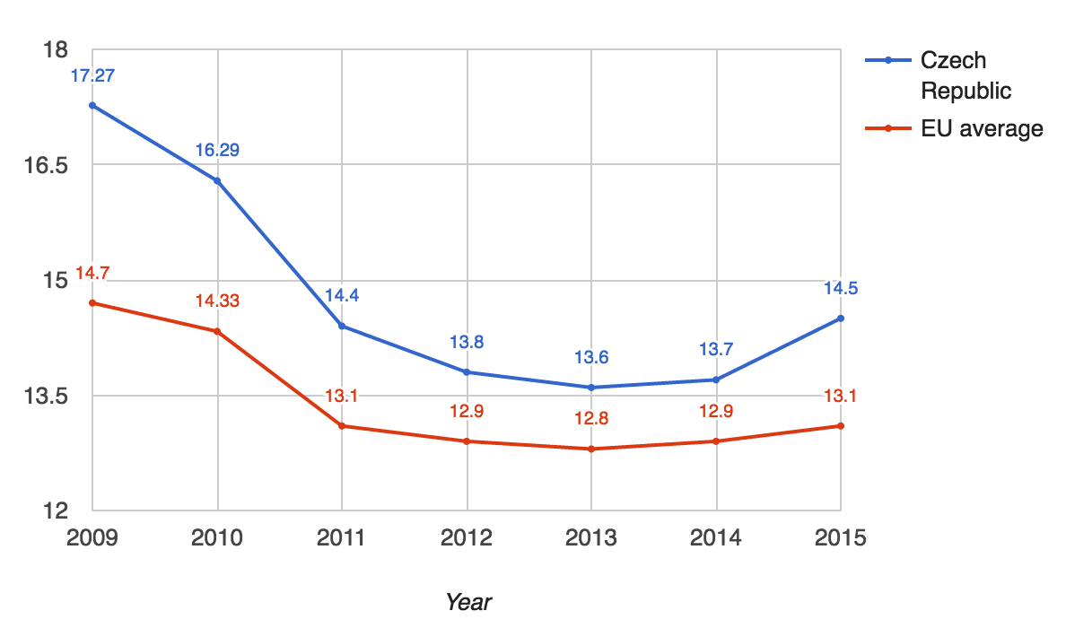
Public procurement constitutes a large share of the volume of transactions in the economy. The share of expenditures in the EU member states’ public procurement on works, goods, and services (excluding utilities) was estimated to be “13.1 % of the EU GDP in 2015, the highest value for the last 4 years” (European Commission 2016). This estimate amounted to 24.2 billion EUR in 2015 in the Czech Republic, which translated to 14.5 % of the country’s GDP (European Commission 2016). Compared with the EU, the Czech Republic exhibits consistent above-average values of this indicator, as can be seen in Fig. 1.
The large volume of transactions in public procurement gives rise to economies of scale, so that even minor improvements can accrue substantial economic impact, since the scale of operations in this domain provides ample opportunity for cost savings. Publishing open data on public procurement as well as using matchmaking methods can be considered among the examples of such improvements, which can potentially increase the efficiency of resource allocation in the public sector, as mentioned in Section 1.4.1.
Due to the volume of the public funds involved in public procurement, it is prone to waste and political graft. Wasteful spending in public procurement can be classified either as active waste, which entails benefits to the public decision maker, or as passive waste, which does not benefit the decision maker. Whereas active waste may result from corruption or clientelism, passive waste proceeds from inefficiencies caused by the lack of skills or incentives. Although active waste is widely perceived to be the main problem of public procurement, a study of the Italian public sector (Bandiera et al. 2009, p. 1282) observed that 83 % of uneconomic spending in public procurement can be attributed to passive waste. We therefore decided to focus on optimizing public procurement where most impact can be expected. We argue that matchmaking can help improve the public procurement processes cut down passive waste. It can assist civil servants by providing relevant information, thus reducing the decision-making effort related to public procurement processes. We identified several use cases in public procurement where matchmaking can help.
1.5.3 Use cases for matchmaking
Matchmaking covers the information phase of market transaction (Schmid and Lindemann 1998, p. 194) that corresponds to the preparation and tendering stages in public procurement life-cycle (Nečaský et al. 2014, p. 865). During this phase “participants to the market seek potential partners” (Di Noia et al. 2004), so that public bodies learn about relevant bidders and companies learn about relevant open calls. In this sense, demands for products and services correspond to information needs and the aim of matchmaking is to retrieve the information that will satisfy them. Several use cases for matchmaking follow from the public procurement legislation according to the procedure types chosen for public contracts, such as:
- Matching bidders to suitable contracts to apply for in open procedures
- Matching relevant bidders that contracting authorities can approach in closed procedures
- Matching similar contracts to serve as models for a new contract
The following use cases are by no means intended to be comprehensive. They illustrate the typical situations in which matchmaking can be helpful.
Public procurement law defines types of procedures that govern how contracting authorities communicate with bidders. In particular, procedure types determine what data on public contracts is published, along with specifying who has access to it and when it needs to be made available. The procedure types can be classified either as open or as restricted. Open procedures mandate contracting authorities to disclose data on contracts publicly, so that any bidders can respond with offers. In this case, contracting authorities do not negotiate with bidders and contracts are awarded solely based on the received bids. Restricted procedures differ by including an extra screening step. As in open procedures, contracting authorities announce contracts publicly, but bidders respond with expression of interest instead of bids. Contracting authorities then screen the interested bidders and send invitations to tender to the selected bidders.
The chosen procedure type determines for which users is matchmaking relevant. Bidders can use matchmaking both in case of open and restricted procedures to be alerted about the current business opportunities in public procurement that are relevant to them. Contracting authorities can use matchmaking in restricted procedures to get recommendations of suitable bidders. Moreover, in case of the simplified under limit procedure, which is allowed in the Czech Republic for public contracts below a specified financial threshold, contracting authority can approach bidders directly. In such case, at least five bidders must be approached according to the act no. 2016/134 (Czech Republic 2016). In that scenario, matchmaking can help recommend appropriate bidders to interest in the public contract. There are also other procedure types, such as innovation partnership, in which matchmaking is applicable to a lesser extent.
An additional use case for similarity-based retrieval employed by matchmaking may occur during contract specification. The Czech act no. 2016/134 (Czech Republic 2016) suggests contracting authorities to estimate contract price based on similar contracts. In order to address this use case, based on incomplete descriptions of contracts matchmaking can recommend similar contracts, the actual prices of which can help estimate the price of the formulated contract.
1.6 Matchmaking
Matchmaking is an information retrieval task that ranks pairs of demands and offers according to the degree to which the offer satisfies the demand. It is a “process of searching the space of possible matches between demand and supplies” (Di Noia et al. 2004, p. 9). For example, matchmaking can pair job seekers with job postings, discover suitable reviewers for doctoral theses, or match romantic partners.
Matchmaking recasts either demands or offers as queries, while the rest is treated as data to query. In this setting, “the choice of which is the data, and which is the query depends just on the point of view” (Di Noia et al. 2004). Both data describing offers and data about demands can be turned either into queries or into queried data. For example, in our case we may treat public contracts as queries for suitable bidders, or, vice versa, bidder profiles may be recast as preferences for public contracts. Matchmakers are given a query and produce \(k\) results best-fulfilling the query (Di Noia et al. 2007, p. 278). Viewed from this perspective, matchmaking can be considered a case of top-\(k\) retrieval.
Matchmaking typically operates on complex data structures. Both demands and supplies may combine non-negotiable restrictions with more flexible requirements or vague semi-structured descriptions. Descriptions of demands and offers thus cannot be reduced to a single dimension, such as a price tag. Matchmakers operating on such complex data often suffer from the curse of dimensionality. It implies that linear increase in dimensionality may cause an exponential growth of negative effects. Complex descriptions make demands and offers difficult to compare. Since demands and supplies are usually complex, “most real-world problems require multidimensional matchmaking” (Veit et al. 2001). For example, matchmaking may involve similarity functions that aggregate similarities of individual dimensions.
Our work focuses on semantic matchmaking that requires a semantic level of agreement between offers and demands. In order to be able to compare descriptions of offers or demands, they need to share the same semantics (González-Castillo et al. 2001). Semantic matchmaking thus describes both queries and data “with reference to a shared specification of a conceptualization for the knowledge domain at hand, i.e., an ontology” (Di Noia et al. 2007, p. 270). Ontologies give the descriptions of entities involved in matchmaking comparable schemata. Data pre-processing may reformulate demands and offers to be comparable, e.g., by aligning their schemata. In order to be able to leverage the semantic features of data, our approach can be thus regarded as schema-aware, as opposed to schema-agnostic matchmaking
Matchmaking overlaps with recommender systems in many respects. Both employ similar methods to achieve their task. However, “every recommender system must develop and maintain a user model or user profile that, for example, contains the user’s preferences” (Jannach et al. 2010, p. 1). Instead of using user profiles, matchmaking uses queries. Although this is a simplifying description and the distinction between matchmaking and recommender systems is in fact blurry, designating our work as matchmaking is more telling.
Besides the similarities with recommender systems, matchmaking may invoke different connotations, as the term is used in other disciplines that imbue it with different meanings. For instance, it appears in graph theory naming the task of producing subsets of edges without common vertices. To avoid this ambiguity, in this text we will use the term “matchmaking” only in the way described here.
We adapted two general approaches for matchmaking: case-based reasoning and statistical relational learning. Both have many things in common and employ similar techniques to achieve their goal. Both learn from past data to produce predictions that are not guaranteed to be correct. A more detailed comparison of case-based reasoning with machine learning is in Richter and Weber (2013, p. 531).
1.6.1 Case-based reasoning
Case-base reasoning (CBR) is a problem solving methodology that learns from experiences of previously solved problems, which are called cases (Richter and Weber 2013, p. 17). A case consists of a problem specification and a problem solution. Experiences described in cases can be either positive or negative. Positive experiences propose solutions to be reused, whereas the negative ones indicate solutions to avoid. For example, experiences may concern diagnosing a patient and evaluating the outcome of the diagnosis, which may be either successful or unsuccessful. Cases are stored and organized in a case base, such as a database. Case base serves as a memory that retains the experiences to learn from.
The workings of CBR systems can be described in terms of the CBR cycle (Kolodner 1992). The cycle consists of four principal steps a CBR system may iterate through:
- Retrieve
- Reuse
- Revise
- Retain
In the Retrieve step a CBR system gets cases similar to the query problem. Case bases are thus usually built for efficient similarity-based retrieval. Since descriptions of cases are often complex, computing their similarity may involve determining and weighting similarities of their individual features. For each use case and each feature a different similarity measure may be adopted, which allows to use pairwise similarity metrics tailored for particular kinds of data. This also enables assigning each feature a different weight, so that more relevant features may be emphasized. The employed metrics may be either symmetric or asymmetric. For example, we can use an asymmetric metric to favour lower prices over higher prices, even though their distance to the price in the query is the same. Since the similarity metrics allow fuzzy matches, reasoning in CBR systems is approximate. Consequently, as Richter and Weber argue, the characteristic that distinguishes CBR from deductive reasoning in logic or databases is that “it does not lead from true assumptions to true conclusions” (2013, p. 18).
A key feature of CBR is that similarity computation typically requires background knowledge. While similarity of cardinal features can be determined without it, nominal features call for additional knowledge to assess their degree of similarity. For instance, a taxonomy may be used to compute similarity as the inverse of taxonomic distance between the values of the compared feature. Since hand-coding background knowledge is expensive, and typically requires assistance of domain experts, CBR research considered alternatives for knowledge acquisition, such as using external semantics from linked open data or discovering latent semantics via machine learning.
The retrieved nearest neighbour cases serve as potential sources of a solution to the query problem. Solutions of these cases are copied and adapted in the Reuse step to formulate a solution answering the query. If a solved case matches the problem at hand exactly, we may directly reuse its solution. However, exact matches are rare, so the solutions to matching cases often need to be adapted. For example, solutions may be reused at different levels. We may either reuse the process that generated the solution, reuse the solution itself, or do something in between.
The reused solution is evaluated in the Revise step to assess whether it is applicable to the query problem. Without this step a CBR system cannot learn from its mistakes. It is the step in which CBR may add user feedback.
Finally, in the Retain step, the query problem and its revised and adopted solution may be incorporated in the case base as a new case for future learning. Alternatively, the generated case may be discarded if the CBR system stores only the actual cases.
The CBR cycle may be preceded by preparatory steps described by Richter and Weber (2013). A CBR system can be initialized by the Knowledge representation step, which structures the knowledge contained in cases the system learns from. Cases are explicitly formulated and described in a structured way, so that their similarity can be determined effectively. The simplest representation of a case is a set of feature-value pairs. However, using more sophisticated data structures is common. In order to compute similarity of cases, they must be described using comparable features, or, put differently, the descriptions of cases must adhere to the same schema.
Problem formulation is a preliminary step in which a query problem is formulated. A query can be considered a partially specified case. It may be either underspecified, such that it matches several existing cases, or overspecified, if it has no matches due to being too specific. Underspecified queries may require solutions from the matching cases to be combined, while overspecified queries may need to be relaxed or provided with partial matches.
Overall, the CBR cycle resembles human reasoning, such as problem solving by finding analogies. In fact, the CBR research is rooted in psychology and cognitive science. It is also similar to case law, which reasons from precedents to produce new interpretations of law. Thanks to these similarities, CBR is perceived as natural by its users (Kolodner 1992), which makes its function usually easy to explain.
CBR is commonly employed in recommender systems. Case-based recommenders are classified as a subset of knowledge-based recommenders (Jannach et al. 2010). Similarly to collaborative recommendation approaches, case-based recommenders exploit data about past behaviour. However, unlike collaborative recommenders, “the case-based approach enjoys a level of transparency and flexibility that is not always possible with other forms of recommendation” (Smyth 2007, p. 370), since it is based on reasoning with explicit knowledge. Our adaptation of CBR for matchmaking can be thus considered a case-based recommender.
1.6.2 Statistical relational learning
Statistical relational learning (SRL) is a subfield of machine learning that is concerned with learning from relational data. SRL learns models that “describe probability distributions \(P(\{X\})\) over the random variables in a relational domain” (Tresp and Nickel 2014, p. 1554). Here, \(X\) denotes a random variable and \(\{X\}\) refers to a set of such variables in a relational domain. The learned model reflects the characteristic patterns and global dependencies in relational data. Unlike inference rules, these statistical patterns may not be universally true, but have useful predictive power nonetheless. An example of such pattern is homophily (McPherson et al. 2001), which describes the tendency of similar entities to be related. A model created by SRL is used to predict probabilities of unknown relations in data. In other words, in SRL “the underlying idea is that reasoning can often be reduced to the task of classifying the truth value of potential statements” (Nickel et al. 2012, p. 271).
There are two basic kinds of SRL models: models with observable features and models with latent features. Our work focuses on the latent feature models. Unlike observable features, latent features are not directly observed in data. Instead, they are assumed to be the hidden causes for the observed variables. Consequently, results from machine learning based on latent features are usually difficult to interpret. Latent feature models are used to derive relationships between entities from interactions of their latent features (Nickel et al. 2016, p. 17). Since latent features correspond to global patterns in data, they can be considered products of collective learning.
Collective learning “refers to the effect that an entity’s relationships, attributes, or class membership can be predicted not only from the entity’s attributes but also from information distributed in the network environment of the entity” (Tresp and Nickel 2014, p. 1550). It involves “automatic exploitation of attribute and relationship correlations across multiple interconnections of entities and relations” (Nickel et al. 2012, p. 272). The exploited contextual information propagates through relations in data, so that the inferred dependencies may span across entity boundaries and involve entities that are more distant in a relational graph. Among other things, this feature of collective learning can help cope with modelling artefacts in RDF, such as intermediate resources that decompose n-ary relations into binary predicates.
Collective learning is a distinctive feature of SRL and is particularly manifest in “domains where entities are interconnected by multiple relations” (Nickel et al. 2011). Conversely, traditional machine learning expects data from a single relation, usually provided in a single propositional table. It considers only attributes of the involved entities, which are assumed to be mutually independent. This is one of the reasons that can explain why SRL was demonstrated to be able to produce superior results for relational data when compared to learning methods that do not take relations into account (Tresp and Nickel 2014, p. 1551). These results mark the importance of being able to leverage the relations in data effectively.
Nowadays the relevance of SRL grows as relational data becomes still more prevalent. In fact, many datasets have relational nature. For instance, vast amounts of relational data are produced by social networking sites. Relational data appears in many contexts, including relational databases, ground predicates in first order logic, or RDF.
Using relational datasets is nevertheless challenging, since many of them are incomplete or noisy and contain uncertain or false statements. Fortunately, SRL is relatively robust to inconsistencies, noise, or adversarial input, since it utilizes non-deterministic dependencies in data. Yet it is worth noting that even though SRL usually copes well with faulty data, systemic biases in the data will manifest in biased results produced by this method.
LOD is a prime example of a large-scale source of relational data afflicted with the above-mentioned ills. The open nature of LOD has direct consequences for data inconsistency and noisiness. These consequences make LOD challenging for reasoning and querying. While SRL can overcome these challenges to some extent, they pose a massive hurdle for traditional reasoning using inference based on description logic. Logical inference imposes strict constraints on its input, which are often violated in real-world data (Nickel et al. 2016, p. 28):
“Concerning requirements on the input data, it is quite unrealistic to expect that data from the open Semantic Web will ever be clean enough such that classical reasoning systems will be able to draw useful inferences from them. This would require Semantic Web data to be engineered strongly according to shared principles, which not only contrasts with the bottom-up nature of the Web, but is also unrealistic in terms of conceptual realizability: many statements are not true or false, they rather depend on the perspective taken.” (Hitzler and van Harmelen 2010, p. 42)
To compound matters further, reasoning with ontologies is computationally demanding, which makes it difficult to scale to the larger datasets in LOD. While we cannot guarantee most LOD datasets to be sound enough for reasoning based on logical inference, “it is reasonable to assume that there exist many dependencies in the LOD cloud which are rather statistical in nature than deterministic” (Nickel et al. 2012, p. 271). Approximate reasoning by SRL is well-suited to exploit these dependencies and to address the challenges inherent to LOD. This setup enables logical inference to complement SRL where appropriate. For example, results produced by logical inference can serve as gold standard for evaluation of SRL, such as in case of Nickel et al. (2012), who used rdfs:subClassOf inferences to evaluate a classification task.
We conceived matchmaking via SRL as a link prediction task. Link prediction is “concerned with predicting the existence (or probability of correctness) of (typed) edges in the graph” (Nickel et al. 2016, p. 14). In the context of knowledge graphs, such as LOD, link prediction is also known as knowledge graph completion (Nickel et al. 2016, p. 14). An example application of link prediction is discovery of protein interactions in bioinformatics. Typical cases of link prediction operate on multi-relational and noisy data, which makes the task suitable for SRL. In our case, we predict the link between a public contract and its awarded bidder.
2 Data preparation
A fundamental part of the hereby presented work is preparation of the Czech public procurement dataset enriched with linked data. The prepared dataset was used to evaluate the matchmakers we built as our main contribution. It served as a use case for applied research in the public procurement domain to explore whether the proposed matchmakers provide useful recommendations in a real-world setting.
In this chapter we will describe the data preparation using the framework of Extract-Transform-Load (ETL) (Kimball and Caserta 2004). ETL is a workflow for data preparation that is guided by the principle of the separation of concerns, as indicated by its compound name. It conceptualizes a sequence of data processing steps endowed with a single main responsibility. Each step is further subdivided into smaller steps endowed with a single responsibility. The self-describing nature of RDF can further contribute to cleaner separation of concerns in the ETL workflow, so that the coupling between the steps involved is reduced.
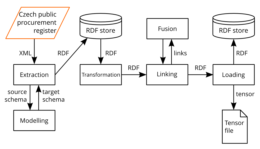
The structure of this chapter roughly follows the steps of ETL. We extend them to modelling, extraction, transformation, linking, fusion, and loading. Modelling produces a target schema, onto which the data is mapped in the course of extraction and transformation. In our setting, extraction refers to the process of converting non-RDF data to RDF. Once data is available in RDF, its processing is described as transformation. Linking discovers co-referent identities, while fusion resolves them to the preferred identities, along with resolving conflicts in data that may arise. Linking and fusion are interleaved and executed iteratively, each building on the results of its previous step. Loading is concerned with making the data available in a way that the matchmaking methods can operate efficiently. The adopted ETL workflow evolved from the workflow that was previously described by this dissertation’s author (2014a). Fig. 2 summarizes the overall workflow.
We employed materialized data integration. Unlike virtual integration, materialized integration persists the integrated data. This allowed us to achieve the query performance required by data transformations and SPARQL-based matchmaking. Our approach to ETL can be regarded as Extract-Load-Transform (ELT). We first loaded the extracted data into an RDF store to make transformation, linking, and fusion via SPARQL Update operations feasible. Using RDF allows to load data first and integrate it later, while in the traditional context of relational databases, data integration typically precedes loading. We used a batch ETL approach, since our source data is published in subsets partitioned per year. Real-time ETL would be feasible if the source data was provided at a finer granularity, such as in the case of the profiles of contracting authorities, which publish XML feeds informing about current public contracts.
Using RDF provides several advantages to data preparation. Since there is no fixed schema in RDF, any RDF data can be merged and stored along with any other RDF data. Merge as union applies to schemas as well, because they too are formalized in RDF. Flexible data model of RDF and the expressive power of RDF vocabularies and ontologies enable to handle variation in the processed data sources. Vocabularies and ontologies make RDF into a self-describing data format. Producing RDF as the output of data extraction provides leverage for the subsequent parts of the ETL process, since the RDF structure allows to express complex operations transforming the data. Moreover, the homogeneous structure of RDF “obsoletes the structural heterogeneity problem and makes integration from multiple data sources possible even if their schemas differ or are unknown” (Mihindukulasooriya et al. 2013). Explicit, machine-readable description of RDF data enables to automate many data processing tasks. In the context of data preparation, this feature of RDF reduces the need for manual intervention in the data preparation process, which decreases its cost and increases its consistency by avoiding human-introduced errors. However, “providing a coherent and integrated view of data from linked data resources retains classical challenges for data integration (e.g., identification and resolution of format inconsistencies in value representation, handling of inconsistent structural representations for related concepts, entity resolution)” (Paton et al. 2012).
Linked data provides a way to practice pay-as-you-go data integration (Paton et al. 2012). The pay-as-you-go principle suggests to reduce costs invested up-front into data preparation, recognize opportunities for incremental refinement of the prepared data, and revise which opportunities to invest in based on user feedback (Paton et al. 2016). The required investment in data preparation is inversely proportional to the willingness of users to tolerate imperfections in data. In our case, we used the feedback from evaluation of matchmaking as an indirect indication of the parts of data preparation that need to be improved.
The principal goal of ETL is to add value to data. A key way to do so is to improve data quality. Since data quality is typically defined as fitness for use, we focus on the fitness of the prepared data for matchmaking in particular. Fitness for this use is affected by several data quality dimensions (Batini and Scannapieco 2006). The key relevant dimensions are duplication and completeness. Lack of duplicate entities reduces the search space that matchmaking has to explore. On the contrary, duplicates break links that can be leveraged by matchmaking. For instance, if there are unknown aliases for a bidder, then data linked from these aliases is unreachable. Incompleteness causes the features potentially valuable for matchmaking to be missing. It makes data less descriptive and increases its sparseness, in turn making matchmaking less effective. However, measuring both these dimensions is difficult. In case of duplication, we can only measure the relative improvement of the deduplicated dataset when compared to the input dataset. Measuring the duplication of the output dataset is unfeasible, since it may contain unknown entity aliases. Similarly, the evaluation of completeness requires either a reference dataset to compare to or reliable cardinalities to expect in the target dataset’s schema. Unfortunately, reference datasets are typically unavailable. Cardinalities of properties either cannot be relied upon or their computation is undermined by unknown duplicates.
While the goals pursued by public disclosure and aggregation of procurement data are often undermined by insufficient data integration caused by heterogeneity of data provided by diverse contracting authorities, ETL can remedy some of the adverse effects of the heterogeneity and fragmentation of public procurement data. However, at many stages of data preparation we needed to compromise data quality due to the effort required to achieve it. We are explicit about the involved trade-offs, because it helps to understand the complexity of the data preparation endeavour. Moreover, for some issues of the data its source does not provide enough to be able to resolve them at all.
Low data quality can undermine both matchmaking as well as data analyses. Data analyses are often based on aggregation queries, which can be significantly skewed by incomplete or duplicate data. Incompleteness of data introduces an involuntary influence of the sampling bias to analyses of such data. For instance, aggregated counts of duplicated entities are unreliable, as they count distinct identifiers instead of counting distinct real-world entities, which may be associated with multiple identifiers. Uncertain quality disqualifies the data from being used scenarios where publishing false positives is not an option. For example, probabilistic hypotheses are of no use for serious journalism, which cannot afford to make possibly untrue claims. Instead, such findings need to be considered as hinting where further exploration to produce more reliable outcomes could be done. On the contrary, in the probabilistic setting of matchmaking even imperfect data can be useful. Moreover, we assume that the impact of errors in data can be partially remedied by the volume of data. Finally, since we follow the pay-as-you-go approach, there is an opportunity to invest more in improving data quality if required.
Preparation of the dataset for matchmaking involved several sources. Selection of each of the data sources had a motive justifying the effort spent preparing the data. We selected the Czech public procurement register as our primary dataset, to which we linked the Common Procurement Vocabulary (CPV), Czech address data, Access to Registers of Economic Subjects/Entities (ARES), and zIndex. The Czech public procurement register provides historical data on Czech public contracts since 2006. CPV organizes the objects of public contracts in a hierarchical structure that allows to draw inferences about the similarity of the objects from their distance in the structure of the vocabulary. Czech address data offers geo-coordinates for the reference postal addresses in the Czech Republic. By matching postal addresses to their canonical forms from this dataset, postal addresses can be geocoded. ARES serves as a reference dataset for business entities. We used it to reconcile the identities of business entities in the Czech public procurement data. zIndex provides a fairness score to contracting authorities in the Czech public procurement. ETL of each of these datasets is described in more detail in the following sections.
The Czech public procurement dataset is available at https://linked.opendata.cz/dataset/isvz. The source code used for data preparation is openly available in a code repository.21 This allows others to replicate and scrutinize the way we prepared data. The data preparation tasks were implemented via declarative programming using XSLT, SPARQL Update operations, and XML specifications of linkage rules. The high-level nature of declarative programming made the implementation concise and helped us to avoid bugs by abstracting from lower-level data manipulation. The work on data preparation started already in 2011, which may explain the diverse choices of the employed tools. Throughout the data preparation, as more suitable and mature tools appeared, we adopted them. A reference for the involved software is provided in Appendix 6.
2.1 Modelling
The central dataset that we used in matchmaking is the Czech public procurement register.22 The available data on each contract in this dataset differs, although generally the contracts feature data such as their contracting authority, the contract’s object, award criteria, and the awarded bidder, altogether comprising the primary data for matchmaking demand and supply. As we described previously, viewed from the market perspective, public contracts can be considered as expressions of demand, while awarded tenders express the supply.
Since public procurement often pursues multiple objectives, public contracts are demands with variable degrees of complexity and completeness. Their explicit formulation thus requires sufficiently expressive modelling, making it a fitting use case for the semantic web technologies, including RDF and RDF Schema. Public contracts may stipulate non-negotiable qualification criteria as well as setting desired, but negotiable qualities sought in bidders. The objects of public contracts are often heterogeneous products or services, that cannot be described only in terms of price. Apart from their complex representation, public contracts have many features unavailable as structured data. These features comprise unstructured documentation or undisclosed terms and conditions. Consequently, matchmaking has to operate on simplified models of public contracts.
We described this dataset with a semantic data model. One key goal of modelling this data was to establish a structure that can be leveraged by matchmaking. However, modelling data in RDF is typically agnostic of its expected use. Instead, it is guided by a conceptual model that opens the data to a wide array of ways to reuse the data. Nevertheless, the way we chose to model our data reflected our priorities.
We focused on facilitating querying and data integration via the data model. Instead of enabling to draw logical inferences by reasoning with ontological constructs, we wanted to simplify and speed-up querying. In order to do that, for example, we avoided verbose structures to reduce the size of the queried data. For the sake of better integration with other data, we established IRIs as persistent identifiers and reused common identifiers where possible. Thanks to the schema-less nature of RDF, shared identifiers allowed us to merge datasets automatically.
The extracted public procurement data was described using a mixture of RDF vocabularies, out of which the Public Contracts Ontology was the most prominent.
2.1.1 Public Contracts Ontology
Public Contracts Ontology23 (PCO) is a lightweight RDF vocabulary for describing data about public contracts. The vocabulary has been developed by the Czech OpenData.cz initiative since 2011, while this dissertation’s author has been one of its editors. Its design is driven by what public procurement data is available, mostly in the Czech Republic and at the EU level. The data-driven approach “implies that vocabularies should not use conceptualizations that do not match well to common database schemas in their target domains” (Mynarz 2014b).
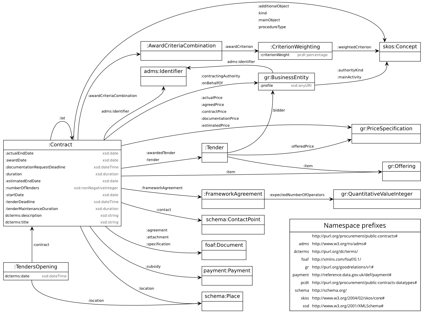
PCO establishes a reusable conceptual vocabulary to provide a consistent way of describing public contracts. This aim for reusability corresponds with the established principle of minimal ontological commitment (Gruber 1993). The vocabulary exhibits a simple snowflake structure oriented around contract as the central concept. It extensively reuses and links other vocabularies, such as Dublin Core Terms24 or GoodRelations.25 While direct reuse of linked data vocabularies is discouraged by Presutti et al. (2016), because it introduces a dependency on external vocabulary maintainers and the consequences of the ontological constraints of the reused terms are rarely considered, we argue that these vocabularies are often maintained by organizations more stable than the organization of the vocabulary’s creator and that the mentioned ontological constraints are typically non-existent in lightweight linked data vocabularies, such as Dublin Core Terms. Several properties in PCO have their range restricted to values enumerated in code lists. For example, there is a code list for procedure types, including open or restricted procedures. These core code lists are represented using the Simple Knowledge Organization System (SKOS) (Miles and Bechhofer 2009) and are a part of the vocabulary. The design of PCO is described in more detail in Klímek et al. (2012) and Nečaský et al. (2014). The class diagram in Fig. 3 shows the Public Contracts Ontology.
The vocabulary was used to a large extent in the LOD2 project.26 For example, it was applied to Czech, British, EU, or Polish public procurement data. In this way, we validated the portability of the vocabulary across various legal environments and ways of publishing public procurement data.
2.1.2 Concrete data model
The concrete data model of the Czech public procurement data uses the PCO mixed with terms cherry-picked from other linked open vocabularies, such as Public Procurement Ontology (PPROC) (Muñoz-Soro et al. 2016), which directly builds upon PCO. The data model’s class diagram is shown in Fig. 4.
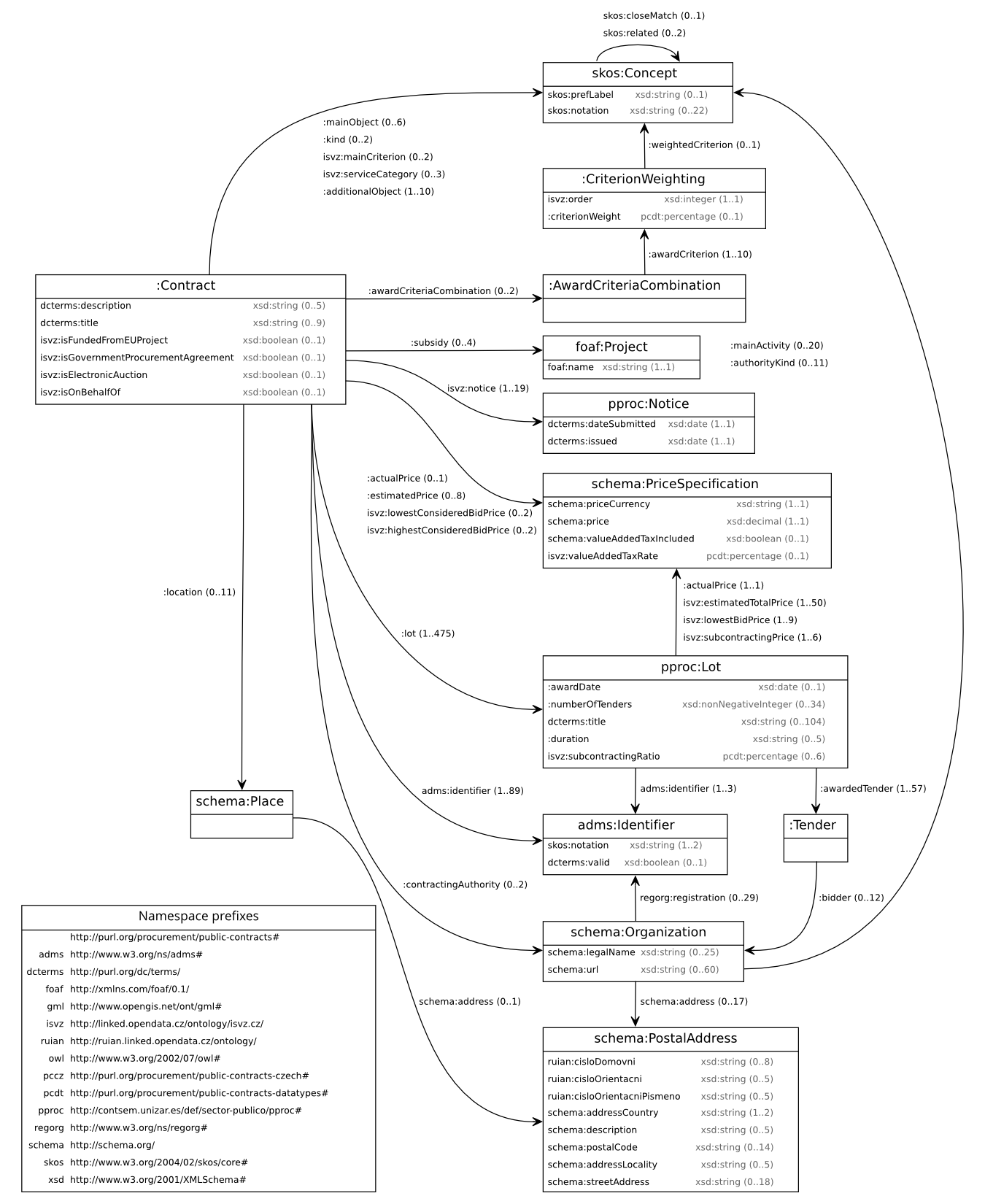
The data model of the extracted data departs from PCO in several ways. There are ad hoc terms in the <http://linked.opendata.cz/ontology/isvz.cz/> namespace to represent dataset-specific features of the Czech public procurement register. Some of these terms are intermediate and are subsequently replaced during data transformation.
Contract objects expressed via pc:mainObject and pc:additionalObject are qualified instead of linking CPV directly. A proxy concept that links a CPV concept via skos:closeMatch is created for each contract object to allow qualification by concepts from the CPV’s supplementary vocabulary. The proxy concepts link their qualifier via skos:related. For example, a contract may have Electrical machinery, apparatus, equipment and consumables; lighting (code 31600000) assigned as the main object, which can be qualified by the supplementary concept For the energy industry (code KA16). This custom modelling pattern was adopted, since SKOS does not recommend any way to represent pre-coordination of concepts.27
Data in the Czech public procurement register is represented using notices, such as prior information notices or contract award notices. Notices are documents that inform about changes in the life-cycle of public contracts. Using the terminology of Jacobs and Walsh (2004), notices can be considered information resources describing contracts as non-information resources. Information resource is “a resource which has the property that all of its essential characteristics can be conveyed in a message” (Jacobs and Walsh 2004), so that it can be transferred via HTTP. On the contrary, non-information resources, such as physical objects or abstract notions, cannot be transferred via HTTP.
We represent contract notices as instances of the subclasses of pproc:Notice from PPROC, since PCO does not include the concept of a contract notice. PCO treats notices as mere artefacts of the document-based communication in public procurement. Each notice pertains to a single contract, while a contract may link several notices informing about its life-cycle. Notices thus provide a way to represent the temporal dimension of contracts. They serve as time-indexed snapshots tracking the evolution of contracts, based on the notice type and its timestamp. To a large extent, we treat notices as intermediate resources, the data of which are combined to form a unified view of contracts during data fusion. Nevertheless, in focusing on the central concept of the public contract, this modelling approach glances over the temporal dimension of other data. For example, it does not accommodate expressing that a contracting authority was renamed. Neither is it supported by PCO, which was designed as atemporal, since modelling temporal data remains an open research topic.
Apart from reusing the code lists incorporated in PCO, we employed a few others. We extracted the code list standardizing categories of procured services as defined in the EU directive 2004/18/EC (EU 2004). This code list links CPV to the Central Product Classification (CPC).28 We also extracted several code lists enumerating the types of contract notices. The EU-wide standard types of notices, including the prior information notice or the design contest notice, were published in 2004 and updated in 2014, with a few types removed, such as the public works concession, or added, such as the modification notice.29 All these code lists were represented in RDF using SKOS.
The diagram of the concrete data model in Fig. 4 shows the Czech public procurement register data after the steps described in this chapter were applied. As is apparent from the cardinalities of many properties, the dataset’s quality is hardly optimal. Maximum cardinalities of several properties are higher than expected due to several reasons. Some entities were inadvertently merged due to their unreliable identifiers. For example, there are few public contracts that share the placeholder identifier 1. We adopted several heuristic counter-measures to avoid fusing distinct entities, such as in case of the previous example, but we could not ensure the reliability of all identifiers in general. Another cause of the high cardinalities is the incomplete data fusion due to insufficient information needed to decide on which values to drop and which ones to keep. Once the hints for data fusion, such as the semantics or temporal order of contract notices, had been used up, there was no more guidance for preferring particular values. When this happened, we either resorted to random sampling or left the data as it was. Ultimately, further improvements in data quality can be made in line with the pay-as-you-go approach if the invested effort is offset by the gains obtained in matchmaking.
2.2 Extraction
Data from the Czech public procurement register was not initially available as structured data, so that the interested parties had to scrape the data from HTML. The dataset was eventually released as open data.30 The data is published in exports to XML, CSV, and Microsoft Excel, each partitioned by year. However, the dataset exports contain only the past contracts that were already awarded, so they cannot be used for alerting bidders about the relevant opportunities in public procurement. Nevertheless, this historical data can be used for training and evaluation. Although published in structured formats, the data is structured poorly, so we had to spend substantial effort improving its structure. The portal publishing this open data also includes exports from the electronic marketplaces where some public contracts are published, such as purchases of commodities. Nonetheless, we did not use this dataset, since it follows a different schema than the Czech public procurement register, so that using it would require us to spend further effort on data preparation. Unfortunately, since data preparation is not a routine task, reliable estimates of the required effort are difficult to come by, so we avoid making them.
We chose the XML version as the source for data extraction. XML allows us to leverage mature tooling, such as XSLT processors, for the extraction. The choice of the input data format also enabled us to explore the data by using the tools designed for manipulating XML.
Ad hoc exploratory queries were done using XQuery. We ran queries to discover possible values of a given XML element or to verify assumptions about the data. Finding distinct values of XML elements helped us detect fixed enumerations, which can be turned into code lists. Queries verifying our assumptions about the data allowed us to tell if an error in data is present in its source or if it is made during data transformation. For example, we assumed that the awarded bidder’s registered identification number (RN) is always different from the contracting authority’s RN. This assumption turned out to be false, caused by errors in the source data.
More systematic analysis of the dataset’s structure was implemented using an XSL transformation. For the purposes of development of the XSL stylesheet we implemented a transformation that computes the cardinalities of elements in the data. This allowed us to tell the always-present elements that can be used as keys identifying the entities described in the data. The tree of element cardinalities revealed the empirical schema of the data. When we looked at this schema, we saw that it follows a fixed structure. In fact, it exhibited a reductive use of XML. Cardinalities of all XML elements were strictly one-to-one, at the expense of empty elements for missing values. Instead of repeating an element in case of multiple values, each value was encoded in a different element named with a numerical index (e.g., <element_1>, <element_2> etc.). For instance, this pattern is used for award criteria, which are represented using the elements <Kriterium1>, <Kriterium2>, etc. Due to the fixed cardinalities, there were many empty elements of this type where less than the maximum number of values was present. To reduce the size of the processed data and simplify further processing we first applied an XSL transformation to remove the empty elements from the data. Doing so simplified the subsequent transformations, since they did not have to cater for the option of empty elements.
We developed an XSL stylesheet to extract the source XML data to RDF/XML (Gandon and Schreiber 2014). The stylesheet maps the schema of the source data onto the target schema described in Section 2.1.2. During the extraction we validated the syntax of registered identification numbers, CPV codes, and literals typed with xsd:date. If possible, we established links in the extracted data by concatenating unambiguous identifiers to namespace IRIs. However, the majority of linking was offloaded to a dedicated phase in the ETL process, covered in Section 2.4, since it typically required queries over the complete dataset. A trade-off we had to make due to our choice of an RDF store was to use plain literals in place of literals typed with xsd:duration, since Virtuoso31 does not yet support this data type. We used LinkedPipes-ETL (LP-ETL) (Klímek et al. 2016) to automate the extraction. LP-ETL provided us with a way to automate downloading and transforming the source data in a data processing pipeline. The syntax of the extracted output was validated via Apache Jena’s riot32 to avoid common problems in RDF/XML, such as incorrect striping (Brickley 2002).
The selected dataset spans Czech public contracts from June 1, 2006 to January 18, 2017. This selection amounts to 1.6 GB of raw data in XML and corresponds to 20.5 million extracted RDF triples. The dataset contains 186 965 public contracts.
To aid the visual validation of the extracted data, we developed sparql-to-graphviz33 that produces a class diagram representing the empirical schema of the data it is provided with. It generates a description of the dataset’s class diagram in the DOT language, which can be rendered to images via Graphviz,34 an established visualization software for graph structures. The dataset’s summary in the diagram, shown in Fig. 4, contains the classes instantiated in the dataset, along with their datatype properties and object properties interconnecting the classes. Each property is provided with its most common range, such as xsd:date for a datatype property or schema:Organization for an object property, and its minimum and maximum cardinality. As mentioned before, the cardinality ranges may signalize errors in the data transformation, such as insufficient data fusion when the maximum cardinality surpasses an expected value.
2.3 Transformation
Since we practiced the principle of separation of concerns, the data extraction produced only intermediate data. This data needed to be transformed in order to reach a better quality and conform with our target data model.
Even though the current documentation of the Czech public procurement register states that the collected data is validated by several rules, we found errors in the data that should have been prevented by the rules. A possible explanation for this issue is that the extracted dataset contains historical data as well, some of which might date to the past when the register did not yet employ as comprehensive validation as it does now. Alternatively, the “errors in the published data may be caused by either negligence when filling out Journal forms or by deliberate obfuscation of sensitive information in order to reduce a contract’s traceability” (Soudek 2016a). A large part of data transformation was therefore devoted to denoising. We dealt both with natural noise, such as the involuntarily introduced typos in literals, and likely malicious noise, such as deliberate omissions to obfuscate the data. Many other data quality problems of the Czech public procurement register are documented on the wiki of zIndex (Soudek 2016a). Similar problems in public procurement data were witnessed by Futia et al. (2017) in case of Italian procurement.
Due to the messiness of the data, we had to make the data transformations defensive. The transformations needed to rely on fewer assumptions about the data and had to be able to deal with violations of these assumptions. For example, the identifiers of the entities involved in public procurement had to be treated as inherently unreliable.
Since not all data is disclosed, we must assume that we have only a sample instead of the complete data. Moreover, given the incentives not to publish data, we cannot assume the sample is random. There may be systemic biases, such as particular kinds of contracting authorities not reporting public contracts properly. Therefore, in general, the findings from the sample cannot be extrapolated to generally valid findings without considering the biases.
2.3.1 Challenges
The key challenges of the data transformation were dealing with high heterogeneity of the data and achieving a workable performance of complex transformations affecting large subsets of data. Due to the volume of processed data and the complexity of the applied transformations, we have not used LP-ETL to orchestrate the transformations. LP-ETL materializes the output of each processing step and, in case of RDF, loads data into an in-memory RDF store, which leads to performance problems when working with higher volumes of data. Nonetheless, LP-ETL allows to execute SPARQL Update operations on data partitioned into chunks of smaller size, which can significantly speed up processing of larger datasets. However, this technique can be used only for transformations that require solely the data present in the chunk, which prevents it from being used in cases the whole dataset is needed by a transformation; e.g., for joins across many resources. An example where this technique is applicable is sequential processing of tabular data, in which data from each row can be processed separately in most cases. Because of its relational nature, our dataset cannot be effectively split to allow executing many kinds of transformations on smaller chunks of data.
Instead of partitioning data, we partitioned the intermediate query bindings in SPARQL Update operations. Transformations using this technique follow the same structure. They contain a sub-query that selects the unprocessed bindings; either by requiring the bindings to match a pattern that is present only in the unprocessed data, e.g., using FILTER NOT EXISTS to eliminate bindings that feature data added by the transformation, or by selecting subsequent subsets from the sorted bindings. For instance, a transformation of instances of schema:PostalAddress can be divided into transformations of non-overlapping subsets of these instances. The latter option for filtering the unprocessed bindings cannot be used when the set of sorted bindings is modified during the transformation. For example, when a transformation deletes some bindings, the offsets of subsets in the ordered set cease to be valid. Additionally, since sorting a large set is a computationally expensive operation, this option may require the sub-query projecting the ordered bindings to be wrapped in another sub-query to be able to cache the sorted set, such as with the Virtuoso’s scrollable cursors.35 The selected unprocessed bindings from the sub-query are split into subsets by setting a limit. The outer update operation then works on this subset and transforms it.
We developed sparql-unlimited36 that allows to run SPARQL update operations following the described structure using Virtuoso. This tool executes transformations rendered from Mustache37 templates that feature placeholders for LIMIT, and optionally OFFSET. Limit determines the size of a subset to be transformed in one update operation. In this way, the processed subset’s size can be adjusted based on the complexity of the transformation. Updates are executed repeatedly, the offset being incremented by the limit in each iteration, until their response reports zero modifications. This stopping condition is Virtuoso-specific, since the SPARQL 1.1 Update standard (Gearon et al. 2013) leaves it unspecified, so that SPARQL engines differ in how they indicate zero modifications. Additionally, sparql-unlimited provides a few conveniences, including configurable retries of failed updates or the ability to restart transformations from a specified offset.
While sparql-unlimited was used to automate parts of individual transformations, each transformation was launched manually. Virtuoso, the RDF store in which we executed the transformations, has an unpredictable runtime, which may be due to unresolved previous transactions or generally faulty implementation. Therefore, we started each transformation manually to allow to fine-tune the configuration for each run depending on the received response from Virtuoso.
A good practice in ETL is to make checkpoints continuously during data processing. Checkpoints consist of persisting the intermediate data output from the individual processing steps, usually to disk. However, due to the large numbers of transformations in our case large disk space would be required if checkpoints were done for every transformation. To reduce disk consumption we persisted only the outputs of the major sub-parts of the data processing pipeline.
2.3.2 Transformation tasks
Overall, we developed tens of SPARQL Update operations for the data transformation. One of the principles we followed was to reduce data early in order to avoid needless processing in the subsequent transformation steps. For example, we deleted empty contract lots and the resources orphaned38 in other transformations. Several transformations were used to clean malformed literals; for example to regularize the common abbreviations for organizations types or convert \/ into V. We removed award dates from the future. We added default values into the data. Since the dataset is of Czech origin, we used Czech koruna (CZK) as the default value in case currency was missing. The addresses without an explicitly stated country were assumed to be located in the Czech Republic. Nonetheless, it is important to acknowledge that adding default values was a trade-off favouring coverage over accuracy.
We paid particular attention to structuring postal addresses in order to improve the results of the subsequent geocoding, described in Section 2.4.5. The primary aim of the transformation of postal addresses was to minimize their variety to increase their chance for match with the reference postal addresses. We managed to extract postal codes, house numbers, and street names from otherwise unstructured data. Accidental variations in postal addresses, such as punctuation, were normalized where possible. Unfortunately, this effort was hindered by a Virtuoso’s bug in support for non-ASCII characters,39 which prevented us from using SPARQL Update operations with diacritical characters, for example when expanding Czech abbreviations in street names.
We made several transformations to move data of select properties, which was difficult to achieve in XSLT during the data extraction. Since RDF/XML lacks a way to express inverse properties, we minted provisional properties in the data extraction, which were reversed as part of the data transformation. For example, a temporary property :isLotOf linking lots to contracts was reversed to pc:lot from PCO. We also corrected domains of some properties, because moving them in XSLT would require joins based on extra key indices.
Some data transformations required additional data. A subset of these transformations leveraged background knowledge from vocabularies. For example, we used rdfs:subClassOf axioms from PPROC to distinguish subclasses of pproc:Notice, when we merged data from notices to contracts. We loaded the required vocabularies into separate named graphs via the SPARQL Update LOAD operation.
In order to make prices comparable, we converted non-CZK currencies to CZK via exchange rates data from the European Central Bank (ECB).40 This dataset contains daily exchange rates of several currencies to EUR. We used an RDF version of the dataset41 prepared for the OpenBudgets.eu42 project. This derivative covers the rates from November 30, 1999 to April 7, 2016, so it allowed to convert most prices in our dataset. Prices in non-CZK currencies were converted using the exchange rates valid at their notice’s publication date. This was done as a two-step process, first converting the prices to EUR followed by the conversion to CZK. In order to automate the execution of this task we employed sparql-to-csv,43 a tool that we developed, which allows to pipe query results into another query or update operation.
The normalized prices were winsorized44 at 99.5th percentile to remove the likely incorrect extreme prices. Due to the limited expressivity of SPARQL this task needed to be split into two SPARQL queries followed by a SPARQL Update operation. The first query retrieved the count of 0.5 % prices, the second query chose the minimum price in the highest 0.5 % prices using the count as a limit, and the final update capped the 0.5 % of highest prices at this minimum. As in the case of currency conversion, we automated the steps of this task using piped queries in sparql-to-csv.
Finally, some estimated prices are expressed as ranges from minimum to maximum price. These prices were converted to arithmetic averages to simplify further processing.
2.4 Linking
Linking is a process of discovering co-referent identifiers. Co-referent identifiers share the same referent, i.e. they refer to the same entity. The existence of co-referent identifiers is possible because linked data operates under the non-unique name assumption (non-UNA). This assumption allows to publish distributed data without the coordination required for agreeing on names. However, queries and data analyses usually operate under the unique name assumption (UNA), and therefore they require a unified dataset without aliases for entities. Consequently, the aim of linking is to discover explicit links between the non-unique names of entities, so that these entities can be unified in data fusion. In this way, linking addresses the accidental variety of data published on the Web.
2.4.1 Content-based addressing
In the absence of agreed-upon identifiers, entities are referred to by their description. Moreover, unlike RDF, some data formats, such as CSV, do not have a mechanism for linking. The lack of shared identifiers established by a reliable authority leads to proliferation of aliases for equivalent entities. Missing consensual identifiers are one of the key challenges in integration of public procurement data (Alvarez-Rodríguez et al. 2014).
If the descriptions with which entities are referred to are reliable and complete, we can use content-based addressing to discover which descriptions refer to the same entity. Content-based addressing is a general approach for identifying entities by using the content of their representations. In case of RDF entities, we assume that triples containing an entity’s identifier as subject or object to make up the entity’s description, also known as the concise bounded description (Stickler 2005). We typically restrict such triples to those in which an entity’s identifier is in the subject role. Various content signatures may be derived from such descriptions of entities.
Simple keys of entities can be derived from values of specific properties. In case of subjects, their keys can be objects of outbound properties that may be interpreted as inverse functional properties; i.e. instances of owl:InverseFunctionalProperty. For example, the property foaf:homepage, which describes an entity’s home page, is defined as an inverse functional property and as such it is usable as a simple key of an entity. In case of objects, their keys can be subjects of inbound properties that may be interpreted as functional object properties; i.e. instances of both owl:FunctionalProperty and owl:ObjectProperty. For example, the property pc:contractingAuthority, which links a contract to its contracting authority, is defined as a functional object property, so that its subject can function as a simple key of the contracting authority. Both kinds of simple key properties may be chained in property paths and followed to obtain keys that do not directly describe the entities they identify. For example, the property path pc:awardedTender/pc:bidder can be treated as a functional object property, the subject of which may be used as a bidder’s key if we accept the assumption that a contract can be awarded to a single organization only. Simple keys are typically used directly as part of entity IRIs, which prevents creating multiple aliases for the entities in the first place. A caution must be given if schema axioms related to functional and inverse functional properties are unreliable or if instance data is diverging from them. In such case, it is better to skip inferring equivalence links via the described methods in order to avoid false results.
Compound keys are more complex content signatures that can be derived from combinations of values of specific properties. In order to be eligible as keys, these combinations must be unique. For example, a contract and a lot number can serve as a compound key for a contract lot. Similarly to simple keys, such compound keys are commonly used as parts of IRIs of the entities they identify. We also employed this approach to merge the bidders sharing the same name and awarded with the same contract. Nevertheless, compound keys are perhaps used more often in a probabilistic setting, in which the degree of their match implies a probability of equivalence of the keyed entities. Fuzzy matches of combinations of values can approximate exact matches of simple keys. However, unlike identifying simple keys, identification of suitable compound keys and approaches for their matching usually requires an expert insight into the domain in question. A common scenario for probabilistic matching of compound keys uses combinations of simple keys that are unreliable identifiers on their own. In the context of our dataset, even when registered identification numbers (RNs) are available, they may be misleading as identifiers. For example, there are several public contracts each year that a contracting authority awards to itself according to the supplied RNs of the authority and the awarded bidder. Moreover, many RNs in the data are syntactically invalid and cannot be automatically coerced to the correct syntax. So, for example, an organization’s name may be combined with its syntactically invalid RN to produce an approximate compound key.
Further extending the size of keys, we can use the complete descriptions of the keyed entities. Since such keys may be unwieldy, they can be substituted by their hashes to make them more manageable. Using hashes as keys is standard in content-based addressing. Hash functions, such as MD5, map variable length descriptions to a fixed length, while preserving their uniqueness. Unlike the previously described approaches for deriving keys, hashes do not require background knowledge to select the key properties, so their production can be fully automated. However, on the one hand, hash keys tend to be more brittle, since any change in the hashed descriptions produces a different hash, which may lead to many false negatives when comparing hashes. On the other hand, hashes can also produce false positives if they are used for underspecified entities. For example, postal addresses for which we know only that they are located in the Czech Republic are unlikely to be the same. The risk of false positives can be reduced by requiring a minimum description, similar to a compound key, to be present. For instance, we can hash only the postal addresses that feature at least a street address and an address locality.
We also experimented with linking entities by discovering entities that are described with a subset of another entity’s description. Given some minimum description of entities to avoid false positives, we assumed that if a set of property-object pairs of a subject is a subset of such set of another subject, the subjects are co-referent. However, detecting subsets in SPARQL is problematic because defining subsets requires universal quantification. Since SPARQL is based on existential quantification instead, universally qualified predicates need to be reimplemented as double negation via nested FILTER NOT EXISTS clauses. Ultimately, we abandoned this linking method because of its poor performance, which makes it unusable for larger data.
In case of entities for which no key can be used to construct IRIs directly during data extraction via XSLT, we employed blank nodes as identifiers. Subsequently, we converted these blank nodes to hash-based IRIs via SPARQL Update operations. The hashes were computed by concatenating the properties and objects of the identified subject and deriving an SHA1 hash from the concatenated string. We used this approach primarily for entities that can be interpreted as structured values, such as price specifications. The entities identified by blank nodes were processed in their inverse topological order. If a blank node linked another blank node, the linked blank node was rewritten first. This was done to ensure that the hashed descriptions of blank nodes do not contain blank nodes, which would cause different hashes to be computed from otherwise equivalent descriptions. Since no two blank nodes are the same, this procedure led to a significant reduction of aliases.
2.4.2 Linking technologies
We employed four kinds of linking technologies. Simple keys and some compound keys were used directly to construct IRIs in XSLT. Linking based on hashes was done using SPARQL Update operations (Gearon et al. 2013). Update operations were also used when creating links required a join via a key, for example when reconciling code list values. Most linking tasks based on fuzzy matches of compound keys were done using the Silk link discovery framework (Bryl et al. 2014). Silk was used when links could not be established via exact matches. For example, we used it to compare syntactically invalid RNs via string distance metrics. We used Silk Workbench, a graphical user interface for Silk, for iterative development of the linkage rules. Silk Workbench displays the results of linking in a way the interlinked entities can be compared manually. This enables to examine a sample of links for false positives and negatives and adjust the linkage rules accordingly, tuning weights and thresholds to avoid the undesired results. An example linkage rule in Silk Workbench is shown in Fig. 5. Elasticsearch45 was employed for matching postal addresses to reference addresses from the Czech addresses dataset.
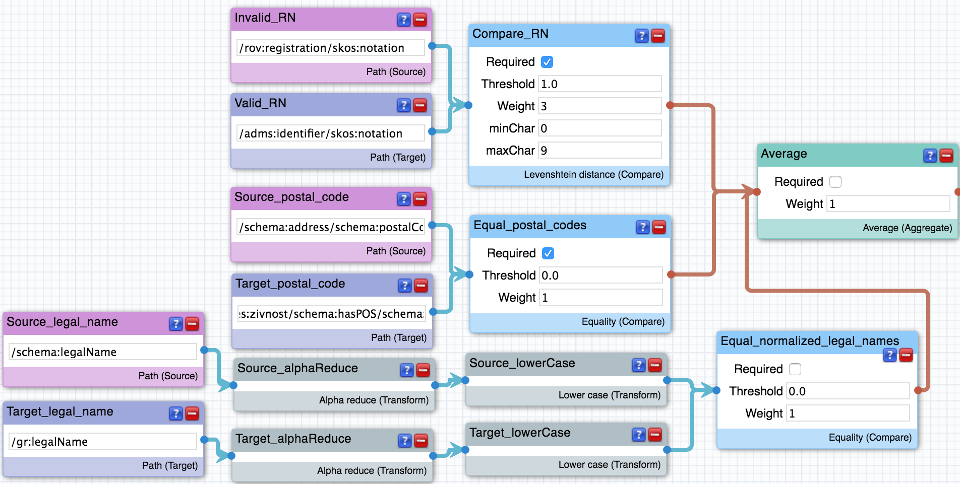
In general, linking was done iteratively, interposed with data fusion. Fusion reduced the size of the data, in turn reducing the search space for linking. Additionally, linking that followed fusion could build on the previously created links.
2.4.3 Linking tasks
We worked on three main linking tasks. We reconciled the values in our dataset with standard code lists. Code lists provide common reference concepts with which values from our source data can be linked. For instance, we mapped different wordings of procedure types to the PCO’s code list for the procedures recognized by the Czech public procurement law.
We linked organizations in the Czech public procurement register to ARES. Instead of deduplicating organizations directly in the public procurement dataset, we decided to reconcile them with ARES, which provided reference identities for organizations. We developed Silk linkage rules using combinations of several properties as compound keys. Syntactically invalid RNs were matched with valid RNs using the Levenshtein string distance metric to find the RNs containing typos. Normalized legal names of organizations were compared via the Jaro-Winkler distance metric with a high required similarity threshold. This metric was selected because it penalizes mismatches near the start of the name more than mismatches at the end. It also takes the lengths of the compared names into account, so that more mismatches are tolerated in longer names. Thanks to these features this distance metric is widely used when comparing names. Legal names were first normalized by converting to lowercase and removing both non-alphanumeric characters and stop-words (e.g., “Czech”), which were generated from the most frequent words appearing in the legal names. Exact matches via postal codes or normalized URLs of organizations were used to disambiguate homonymous organization names. Unfortunately, URLs were discovered to be unreliable as simple keys, because they can be assigned incorrectly, so that we used them as keys only in combination with other data. Geo-coordinates of organizations obtained by geocoding postal addresses were used to filter matches by maximum allowed geographic distance. The resulting equivalence links generated by Silk were serialized using the owl:sameAs property, loaded in a separate named graph, and resolved during data fusion. In total, we generated 6842 links for the 14177 business entities unlinked to reference entities from ARES. Resolution of these links thus reduced the share of the unlinked business entities from 33.38 % to 15.9 %.
We geocoded postal addresses in ARES and in the Czech public procurement register by linking them to the Czech addresses dataset. Geocoding is the described in greater detail further in a separate section.
2.4.4 Evaluation of linking
Evaluation of the quality of linking typically involves a clerical review of a sample of the resulting equivalence links (Christen 2012, p. 174). By using manual assessment, a randomly selected sample of links can be split into correct and incorrect matches. This allows to compute quality metrics, such as precision, which is defined as the ratio of correct links (true positives) to all links (positives). Results of the metrics computed on a sample may be then extrapolated to approximate the quality of the complete output of linking.
We manually evaluated a randomly selected sample of 200 links to ARES generated by approximate matching in Silk. To a limited extent, the evaluation of this subset of links can substitute the evaluation of all links, which was unfeasible due to the manual effort involved in assessing link validity. Validity of each link was confirmed or rejected based on the data published in the PR, also taking into account its changes over time, or based on the web sites of the linked organizations. 9 links were determined to be false positives, while the rest was confirmed to be valid. This ratio of false positives produces the precision of 0.955. We consider such precision to be reasonable, given the low quality of the linked data. Some of the false positives were caused by ambiguous descriptions of business entities. For example, there are two distinct entities named COMIMPEX spol. s r.o. that also share the same organization type.
Apart from the clerical review, there are also few automated measures that may indicate the quality of links. An example of such measure is the reduction ratio, defined as the number of generated equivalence links compared to all possible equivalence links. Effectiveness of linking measured in its total runtime compared to the number of the processed entities can also be determined without human input. A more detailed review of the evaluation methods for linking is presented by Christen (2012, pp. 163–184).
2.4.5 Geocoding
Geocoding is the process of linking postal addresses to geographic locations. The locations are represented as coordinates corresponding to a place on the Earth’s surface. Geocoding can be considered a case of instance matching (Christen 2012, sec. 9.1) that matches addresses from a dataset to reference addresses equipped with geo-coordinates. We geocoded the postal addresses of business entities in the Czech public procurement register, the Public Register (PR), and the Trade Licensing Register (TLR). In case of PR we geocoded only the addresses that were missing links to the Czech addresses dataset. Unlinked addresses in PR amounted for 12.42 % of all its addresses. No addresses in TLR were linked. In total, we geocoded over 180 thousand postal addresses from these registers. In case of the Czech public procurement register we geocoded the addresses of business entities that were not linked to the above-mentioned registers. The overall goal of this effort was to be able to locate the business entities for the purposes of linking, analyses, and matchmaking.
The main challenge to address in geocoding was the lack of structure in the geocoded data. As described in Section 2.3, we attempted to parse the unstructured addresses to recover their structure. Nevertheless, many addresses contained just a name of a region or a municipality. This is why we started with simple geocoding based on matching region or municipality names.
We used LP-ETL to extract the names of regions and municipalities along with their corresponding geo-coordinates from the RÚIAN SPARQL endpoint.46 The data provides geo-coordinates of centroids of each region and municipality. The geo-coordinates were reprojected from EPSG:5514 coordinate reference system (CRS) to EPSG:4326 to improve their interoperability, since the latter one is a de facto standard CRS on the Web. We loaded the data into our RDF store and ran a SPARQL Update operation to match the geo-coordinates to postal addresses via the names of regions and municipalities.
In order to geocode other postal addresses, we built an Elasticsearch-based geocoder using the Czech addresses data, covered in Section 2.4.6.3. We decided not to use an existing solution for several reasons. Some existing services for geocoding have restrictive licenses. For instance, the results of the Google Maps Geocoding API can be used only in conjunction with displaying the obtained geo-coordinates on a map from Google Maps.47 More liberal geocoding services often provide poor accuracy. For example, this is the case of OpenStreetMap’s Nominatim,48 both for its structured and unstructured search. Finally, we wanted to assess whether open data can help build a geocoder on par with the commercial offerings. This is why we based the developed geocoder on the gazetteer built from the Czech address data.
During the development of the geocoder we leveraged the tooling we built for data preparation, described in the Appendix 6. sparql-to-jsonld49 was used to retrieve the Czech addresses data from a SPARQL endpoint, construct descriptions of the individual postal addresses, and frame them into JSON-LD documents. We used jsonld-to-elasticsearch50 to index the addresses in Elasticsearch. In the index phase we applied a basic normalization and employed a synonym filter to expand the abbreviations commonly found in postal addresses.
The geocoder elasticsearch-geocoding51 was implemented as a command-line tool that loads the addresses to geocode from a SPARQL endpoint using a paged SPARQL SELECT query provided by the user, and queries an Elasticsearch index with the Czech addresses data for each address. We adopted Elasticsearch for the geocoder because, unlike SPARQL, it allows to perform fuzzy searches, in which results are ranked by the degree to which they fulfil the search query. This is useful since the geocoded addresses may be incomplete, poorly structured, or contain misspellings. In case we obtained multiple results from the geocoder, we selected the first one, which ranked the best.
Since we practice separation of concerns, the geocoder expects a reasonably clean input. It is the responsibility of data preparation to structure and normalize the geocoded postal addresses. This effort has benefits for many tasks, not geocoding only. Instead of ad hoc cleaning during geocoding we thus prepared the postal addresses as part of the ETL pre-processing, as described in Section 2.3.
The geocoder generates the queries to Elasticsearch from its input addresses. Since every property of the addresses is optional, the queries can be generated in several ways, depending on the semantics associated with the properties. If schema:description is the only available property, we search for it across all fields. A more complex query matching combinations of subqueries is generated if more properties are present. The objects of postal code (schema:postalCode) and address locality (schema:addressLocality) are treated as co-referent, so that it suffices if one matches if both are available.
The design of the geocoding queries was guided by the level of accuracy required to support the envisioned use cases. For us errors in the range of tens to hundreds of meters are tolerable, so that we could trade in accuracy for increased recall. We made adjustments to the geocoding queries to better serve this objective. As house numbers and orientational numbers are often mixed up, we enabled the geocoding queries to match either number. We boosted the weight of postal codes because the match on their level is more important than the match on more specific levels, such as the house number. Prior to introducing the boost for postal codes, in some cases distant addresses sharing the same street address and house number were mixed in their geolocation. Moreover, unlike address localities, postal codes are usually regular, which makes them more reliable in retrieval. Further optimization of the geocoding queries was guided by the results of evaluation.
2.4.5.1 Evaluation
We chose to evaluate the geocoder by using metrics adapted from Goldberg et al. (2013). Match rate is defined as the share of addresses capable of being geocoded. If \(A\) is a set of addresses and \(geocode()\) is a geocoding function, we can define the match rate \(mr\) as follows:
\[mr = \frac{|\{a \in A, geocode(a) \neq \varnothing\}|}{|A|}\]
We adapted the spatial accuracy metric as the share of addresses that are geocoded within a specified distance from the reference location. We chose to evaluate spatial accuracy at 50 meters, so that geo-coordinates found within 50 meters from the reference location are considered matching. Provided a set of addresses \(A\) and ground truth \(G\) containing the true geo-coordinates, we can define this metric \(sa\) in the following way:
\[sa = \frac{|\{a \in A, distance(geocode(a), G_a)< 50\}|}{|A|}\]
While match rate can be computed without a gold standard dataset, spatial accuracy needs one. Thanks to the links to the Czech addresses dataset from the Public Register, we had a dataset that could be used as a gold standard. Nevertheless, the provenance and quality of these links is undocumented, with a possibility of outdated or invalid links due to mismatched versions of the linked datasets. Therefore, we decided to verify them by comparing them to another datasets. We experimented with several geocoding services, including Google Maps Geocoding API,52 MapQuest Geocoding API,53 and Here Geocoding API,54, to assess their accuracy. Here Geocoding API turned out to deliver the best results while also providing a liberal licence allowing to use its geo-coordinates in our evaluation. When geocoding with this API, we used structured queries with a bounding box set to the Czech Republic to rule out the evident non-matches.
We loaded 10 thousand randomly selected postal addresses from the PR that linked the Czech addresses dataset. Out of this sample, 73 % of the geo-coordinates provided by the Here Geocoding API were found no farther than 1 meter from the source geo-coordinates. In this way, we purified two “silver” standard datasets into a gold one, consisting of 7300 postal addresses with verified geo-coordinates. The match rate achieved by our geocoder on this dataset was 0.9893. The geocoder scored 0.9556 for the spatial accuracy at 50 meters, with median distance of 0.425 meters and mean average distance of 272 meters.
We also evaluated our geocoder using a sample of 5 thousand addresses from the TLR, for which true location was unknown. The geocoder achieved a match rate of 0.9788, while Here Geocoding API scored 0.6278 on this sample. We sorted the postal addresses that were matched both by Here Geocoding API and our geocoder by the distance of the returned geo-coordinates in descending order. We manually checked the top geo-coordinates and found that the maximum distance where our geo-coordinates were invalid was 8 kilometers. The obtained median distance was 0.63 meters and the arithmetic mean distance was 290 meters. We deemed such results to be reasonable for our use case.
2.4.6 Linked datasets
We linked several datasets with the Czech public procurement register. In this section we describe how these datasets were prepared. Fig. 6 shows how these datasets are linked. In this diagram, dataset size corresponds to the number of RDF triples in the dataset, while the thickness of lines between the datasets corresponds to the number of links connecting them. Both proportions are logarithmically scaled for display purposes.
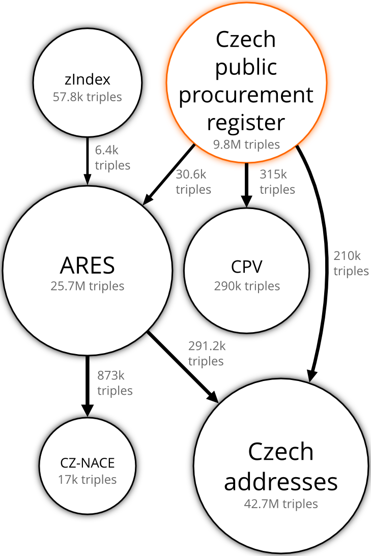
In the following we review these linked datasets and explain how they were obtained and prepared.
2.4.6.1 Common Procurement Vocabulary
Common Procurement Vocabulary (CPV)55 is a controlled vocabulary standardized by the EU for harmonizing the description of procured objects across the EU member states. Within the EU, CPV has been mandatory to use for public procurement since 2006. The most recent version of CPV is from 2008. Each CPV concept is provided with labels in 23 languages of the EU. The multilingual nature of CPV allows to localize public procurement data to support cross-country procurement. CPV consists of the main and the supplementary vocabulary. The main vocabulary provides primary concepts to describe public contracts, such as 90521400 that stands for “Transport of radioactive waste”. There are 9454 concepts in the main vocabulary, structured in 6 levels of hierarchy. The supplementary vocabulary can be used to qualify concepts from the main vocabulary. An example supplementary concept is MF09, meaning “Using hovercraft”. There are 903 concepts in the supplementary vocabulary, organized in a flat list. However, the supplementary vocabulary is rarely used. Only 3.25 % of objects in the Czech public procurement dataset are qualified with a supplementary concept. CPV has a monohierarchical structure in which the individual taxonomic links typically have the flavour of either subsumption56 or part-whole57 relations between the vocabulary’s concepts. The hierarchical structure allows to derive a correspondence between the concept’s location in the structure and its conceptual similarity to its neighbouring concepts, which makes it possible to perform basic reasoning and query expansion.
The monohierarchical design may have caused conceptual duplication within distinct branches of the vocabulary. For instance, there are two concepts labelled as “Transport equipment and auxiliary products to transportation”. One is 34000000, which constitutes its own branch in the vocabulary, and the other is 33952000, which is nested in the branch “Medical equipments, pharmaceuticals and personal care products”. Apart from the sharing same label, there is no explicit link between these concepts. Moreover, CPV is published in tree (XML) or tabular (XLS) data formats, which may have encouraged the vocabulary’s monohierarchical design by making it simpler to implement. Polyhierarchy may solve the duplication by allowing concepts to have multiple parents. However, polyhierarchies are graphs, so RDF is more suitable to represent them.
We may sidestep polyhierachy by creating associative links between similar concepts within different branches of the vocabulary’s hierarchical structure. In this way, graph distance within CPV can better approximate the semantic distance of the compared concepts and allow similarity-based retrieval. In order to achieve this goal, we experimented with link discovery tools to construct associative links within the vocabulary. In the absence of better features to anchor the sense of the concepts, we compared the concepts’ multilingual labels to determine their similarity. Even with the modest size of the vocabulary this exercise turned to be computationally expensive, since it would require over a trillion of pair-wise comparisons due to the number of languages involved. This naïve approach could be improved by using techniques, such as blocking (Isele et al. 2011), however, given its tenuous benefits, we decided to abandon this effort.
In order to integrate CPV with the public procurement data, we converted it from XML to RDF. The transformation58 was done using an XSL transformation and SPARQL CONSTRUCT queries for enriching data. Its result is described using SKOS plus Dublin Core Terms59 for metadata. While the original CPV source expresses hierarchical relations implicitly using the structure of numerical notations of the vocabulary’s concepts, its RDF version makes these relations explicit using hierarchical relations from SKOS, such as skos:broaderTransitive. The transformation was originally orchestrated by a shell script, which was later replaced by a UnifiedViews60 (Knap et al. 2017) pipeline. UnifiedViews is an ETL tool for producing RDF data, which can be considered a predecessor of LP-ETL.
The Czech public procurement register mandates the use of the 2008 version of CPV since September 15, 2008. Since the data we processed goes back to 2006, we had to account for public contracts described with the previous version of CPV from 2003. In order to harmonize the description of the older contracts we used the correspondence table mapping CPV 2003 to CPV 2008 published by the EU Publications Office.61 We developed an LP-ETL pipeline to convert the correspondence table from Excel to CSV and map it to RDF using SKOS mapping relations, such as skos:closeMatch. The following part of the transformation turned out to be problematic. Cells that would duplicate the values of the cells above them were left empty in the source spreadsheet. Therefore, we had to create a “fill down blanks” functionality to duplicate cell values in following directly adjacent empty cells. The SPARQL Update operation implementing this functionality came off as taxing, notwithstanding the modest size of the processed data. LP-ETL had to be abandoned as it could not run the operation to completion. Instead, we adopted Apache Jena’s arq62 that was able to execute it. Provided the RDF version of the mappings from the correspondence table, concepts from CPV 2003 were resolved to their CPV 2008 counterparts by using a SPARQL Update operation that exploited the mappings.
2.4.6.2 Access to Registers of Economic Subjects/Entities
Access to Registers of Economic Subjects/Entities63 (ARES) is an information system about business entities. It is maintained by the Ministry of Finance of the Czech Republic. The data in this system describes business entities along with their registrations required to pursue their business. It contains legal entity names, registration dates, postal addresses, and classifications according to NACE. Thanks to these features ARES can serve as a reference dataset for the Czech business entities.
This system is not the primary source of the data it provides. Instead, it mediates data from several source registers and links back to them where possible. The main sources of ARES are the Public Register64 (PR) run by the Czech Ministry of Justice, the Trade Licensing Register65 (TLR) operated by the Czech Ministry of Industry and Trade, and the Business Register66 (BR) maintained by the Czech Statistical Office (CSO). Consequently, the data ARES provides may not be up-to-date or complete. In fact, ARES explicitly renounces any guarantees about the data. Its data is not to be treated as legally binding, instead, it serves only an informative purpose.
The benefit of ARES that outweighs its drawbacks is that, unlike its source registers, it provides data in a structured format. It exposes an HTTP API67 that allows to retrieve data in XML about one legal entity per request. The access to data is rate-limited to prevent high load from automated harvesters that may cause unavailability of the service for human users. The limits allow to issue a thousand requests per day and five thousand requests per night. Since ARES provides access to hundreds of thousands of business entities and no option for bulk download, harvesting a copy of its data may take many weeks. The rate-limiting and the prolonged execution thus need to be factored into account when designing an ETL pipeline that obtains the data.
Since ARES wraps many registers, we narrowed our focus to two registers most relevant to the public procurement: PR and TLR. These registers are those that the awarded bidders of public contracts are registered in. We used only a subset of BR that links bidders to concepts from the NACE classification. A large share of business entities is present in both PR and TLR. It is nevertheless useful to obtain data from both registers, since they are complementary. For instance, while the PR contains a classification of organization activity, TLR naturally provides the trade licences entities have registered.
Valid requests to the ARES API must contain a Registered Identification Number (RN) of a business entity. This design makes it difficult to obtain a complete copy of the ARES data without a complete list of valid RNs. We collected a subset of the entire datasets by requesting the RNs we found in other datasets. The Czech public procurement register was one such dataset, so we gathered data about all business entities participating in the Czech public procurement if their valid RN was published. The downside of the method is that it potentially leaves out much unidentified business entities, since there are almost 2.8 million business entities in total according to the BR as of September 2016.68 Moreover, this number excludes the now defunct entities that could have been involved in the Czech public procurement before their dissolution date. In total, as of November 2016 we harvested data about 204 620 distinct entities either in PR or TLR. Out of these, 161 403 business entities were present in both registries.
What we made was thus a snapshot of data valid at the harvest date. However, business entities change in time and so does the data in ARES that describes them. For instance, companies may move to different postal addresses. Without the complete history of the registers, access to the previous addresses is unavailable. Since we have obtained only a snapshot of the data, it was missing the historical data. This deficiency turned out to be detrimental to linking business entities by making it more difficult to identify the correct reference entities to link.
Thanks to the uniform API that ARES provides the ETL of both registers differs only in the URL parameters and the XSL transformations that map XML data to RDF. The data transformation was done using UnifiedViews. A custom component of UnifiedViews, called a data processing unit69 (DPU), was used to fetch data from ARES. The raw source data in XML was transformed into RDF/XML by using XSL stylesheets. A mixture of RDF vocabularies was used to describe the ARES data, with the key roles played by the GoodRelations (Hepp 2008) and the Registered Organization Vocabulary (Archer et al. 2013). The retrieved data was relatively consistent, so it did not require much cleaning. However, we paid a special care to cleaning postal addresses, since we needed them for geocoding. SPARQL Update operations were employed to clean and structure the addresses. The data transformation70 was released as open source. Most of the transformation was done by Jakub Klímek from the Charles University in Prague with a contribution of this dissertation’s author, in particular regarding the XSL stylesheets and SPARQL Update operations.
We used a subset of BR containing a classification of the registered business entities. The organizations in BR are assigned concepts from the Statistical Classification of Economic Activities in the European Community (NACE). NACE is a hierarchical classification that describes the economic activities pursued by business entities. A subset of BR in CSV that contained the links to NACE was provided to us via personal communication with Ondřej Kokeš who harvested it from ARES. We extracted 873 thousand links to NACE from this subset and converted them to RDF via Tarql71, a command-line tool for converting tabular data to RDF via SPARQL CONSTRUCT queries. Links to NACE were available for 89.5 % of organizations in the Czech public procurement register that were linked to ARES.
The version of NACE that these links use is CZ-NACE,72 a Czech extension to NACE Rev. 2 that adds specific leaf concepts. CZ-NACE is maintained by the CSO, which provided us with this classification in XML. We converted the source data to RDF by using a custom Python script.
2.4.6.3 Czech addresses
In order to provide the postal addresses in the Czech public procurement data with geo-coordinates, we extracted the Czech addresses data from the Registry of territorial identification, addresses, and real estate73 (RÚIAN). The registry contains 2.9 million addresses74 located in the Czech Republic. The addresses refer to locations of buildings that can be assigned unambiguous addresses.75 Most addresses are provided with representative address points. For example, geo-coordinates of an address point may be located at the entrance of the building its address is assigned to.
The Czech addresses data is available in CSV.76 We used LP-ETL to transform it to RDF. Each address was modelled as an instance of schema:PostalAddress. The RÚIAN-specific attributes, such as the orientational number or the building type, were described with the RÚIAN Ontology previously developed by the OpenData.cz initiative. Since each row in the source data is independent of the others, it was possible to use the chunked transformation in LP-ETL to process smaller batches of rows separately and thus decrease the execution time of the transformation. The resulting data, consisting of 42 million RDF triples, was loaded into a Virtuoso RDF store.
The Czech addresses data uses Systém Jednotné trigonometrické sítě katastrální (S-JTSK)77 as its coordinate reference system (CRS). S-JTSK is based on the Křovák projection, which was designed specifically for the Czechoslovakia to provide more precise geo-coordinates than another reference system would. However, the standard CRS used in web applications is the World Geodetic System (WGS84). Data using S-JTSK is thus not directly interoperable with many existing datasets. If data adhering to multiple coordinate reference systems are to be used together, they must be reprojected to a single CRS to make their geo-coordinates comparable. Reprojection carries with it a loss of precision, but it is minute. The error in the conversion from S-JTSK to WGS84 using a transformation key is below 1 meter. The largest error, close to 1 meter, can be observed for geo-coordinates near the borders of the Czech Republic.78 We therefore decided to trade this minor loss in precision for increased interoperability and reprojected S-JTSK to WGS84.
At the time the data was transformed (September 2016) LP-ETL did not support reprojection of geo-coordinates. In its current version (as of September 2017) it features a component79 that offers this functionality. We thus implemented the reprojection as a separate step following the data transformation in LP-ETL. We developed a command-line tool that requested the original geo-coordinates in paged batches by using SPARQL SELECT queries, reprojected them, and uploaded the batches back to the RDF store using SPARQL Update operations. The geo-coordinates were reprojected via the open source GeoTools80 Java library.
According to its documentation, the Czech addresses dataset uses the EPSG:551481 variant of the S-JTSK CRS since 2011. The variant in use till 2011 was EPSG:2065.82 Contrary to the documentation, we discovered that the reprojection delivered more precise results if EPSG:2065 was used instead of EPSG:5514, when compared to the results of the RÚIAN reprojection service.83 We may ascribe this difference to the precision of the transformation keys that were used for the compared variants. Nevertheless, the differences among the variants ranged in centimeters, so that they were negligible for the purposes we wanted to use the geo-coordinates.
In fact, the reprojection of the Czech addresses geo-coordinates would not be necessary if we only computed distances within this dataset. However, the reprojection was needed in order to be able to compare the geo-coordinates with WGS84 geo-coordinates produced by existing geocoding services for the purpose of evaluation of geocoding, as described in Section 2.4.5. Moreover, the reprojection to a standard coordinate reference system generally improved the ease of use of the data. For example, map visualizations, that are typically done using software libraries expecting WGS84 geo-coordinates, could thus avoid using to on-the-fly reprojections of the data.
2.4.6.4 zIndex
zIndex84 grades Czech contracting authorities with fairness scores. The scores are based on the contracting authority’s adherence to good practices in public procurement as observed from the data it discloses (Soudek 2016b). As its authors suggest, high zIndex score implies that there is less room for mismanagement of public funds, while a low score indicates the opposite. zIndex scores are normalized to the interval between 0 and 1, in which 1 represents the best score. The index is produced by the EconLab,85 a Czech economic NGO focused on public policy.
Our case-based reasoning approach to matchmaking works under the assumption that the awarded bidders constitute cases of successful solutions to public contracts. As we discuss at length further in Section 3.1, this assumption may not be universally valid, considering that bidders may be awarded for reasons other than providing the best offer. zIndex gives us a counter-measure to balance this assumption by weighting each award by the fairness score of its contracting authority.
However, the perceived fairness of contracting authorities may change over time and so do their zIndex scores that are based on a specific period of the contracting authority’s history. In our case, most scores zIndex scores we had were derived from the period from 2011 to 2013. As such, they are most relevant for public contracts dated at the end of this period, and may be misleading for the contracts awarded in years further apart.
zIndex scores were initially supplied to the author by Datlab s.r.o.86 in September 2014. An updated snapshot of zIndex was provided upon request in January 2017. The data in CSV was transformed to RDF by using Tarql. The RDF version of the data was represented as a simple data cube using the Data Cube Vocabulary (Cyganiak and Reynolds 2014). Each zIndex score was modelled as a measure of an observation indexed by the dimensions of the scored contracting authority and the rating period. Contracting authorities in this dataset are identified by their IRIs from ARES, which are automatically derived from their RNs. The scores are available for 29.4 % of the contracting authorities in our dataset.
2.5 Fusion
Data fusion can be defined as “the process of integrating multiple data items representing the same real-world object into a single, consistent, and clean representation” (Bizer et al. 2009). In order to reach this goal, data fusion removes invalid or non-preferred data, so that “duplicate representations are combined and fused into a single representation while inconsistencies in the data are resolved” (Bleiholder and Naumann 2008, p. 1:3). Fusion of RDF data can be considered a counter-measure to the effects of the principle of Anyone can say anything about anything (AAA). As Klyne and Carroll state, “RDF cannot prevent anyone from making nonsensical or inconsistent assertions, and applications that build upon RDF must find ways to deal with conflicting sources of information” (2002).
In line with the principle of separation of concerns, data fusion expects equivalence links between conflicting identities to be provided. However, it is not limited to a mechanical application of the equivalence links produced by linking. Its particular focus “lies in resolving value-level contradictions among the different representations of a single real-world object” (Naumann et al. 2006, p. 22).
Viewed from the perspective of data fusion, linking is a way to discover identity conflicts. Identity conflicts arise when a single entity is provided with multiple identities. Identities in RDF correspond either to IRIs or blank nodes. Resolution of identity conflicts gives rise to data conflicts in turn. Rewriting an identity with another identity automatically merges the RDF triples in which the identities appear. Merging RDF triples may consequently cause functional properties to have multiple values, which constitutes a conflict.
Fusion may be executed iteratively, interleaved with linking. This is expedient in case of large datasets, which are computationally demanding to process. Iterating fusion with linking allows to shrink the size of the processed data and thus decrease the number of comparisons that linking needs to perform. Moreover, in case of large datasets, the steps of linking and data fusion may be limited to subsets of data in order to improve the performance of the whole workflow.
In order to simplify the resolution of identity conflicts, we adopted a conventional directionality of the owl:sameAs links from a non-preferred IRI to the preferred IRI. This convention allowed us to use a uniform SPARQL Update operation to resolve non-preferred IRIs to their preferred counterparts. For example, if there is a triple :a owl:sameAs :b, :a as the non-preferred IRI will be rewritten to :b. Note that this convention is applicable only if you can distinguish between non-preferred and preferred IRIs, such as by preferring IRIs from a reference dataset.
Data conflicts arose only in properties that can be interpreted as functional. Some of these properties explicitly instantiate owl:FunctionalProperty, such as pc:kind describing the kind of a contract, while others, such as dcterms:title expressing the contract’s title, can be endowed with this semantics for the purpose of attaining a unified view of the fused data. Most of our data fusion work was devoted to resolving data from contract notices. As was the case of identity conflicts, the resolution of data conflicts was done via SPARQL Update operations.
Conflicts are resolved by using resolution functions. Resolution functions are either deciding, which pick one of their inputs, or mediating, which derive their output from the inputs. An example deciding function is picking the maximum value, while an example mediating function is computing the median value. We employed deciding conflict resolution functions.
2.5.1 Conflict resolution strategies
The conflict resolution strategies we implemented can be classified according to Bleiholder and Naumann (2006). We used Trust your friends (Bleiholder and Naumann 2006, p. 3) strategy to prefer values from ARES, since we consider it a trustworthy reference dataset. Leveraging the semantics of notice types, we preferred data from correction notices. A similar reason led us to remove syntactically invalid RNs in case valid RNs were present too. We used Keep up to date (Bleiholder and Naumann 2006, p. 3) metadata-based conflict resolution strategy to prefer values from the most recent public notices. We determined the temporal order of notices from their submission dates and the semantics of their types, which represent an implicit order. For example, prior information notice comes before contract notice, which in turn precedes contract award notice. The order of notice types can be learnt from the most common order of notices with immediately following submission dates. We combined such distribution of subsequent notice types with manual assessment to rule out erroneous pairs. The order of notice types was provided as an inline table to the SPARQL Update operation resolving the conflicts. In line with this strategy, we also preferred the most recent values of pc:awardDate. We used Most specific concept (Bleiholder and Naumann 2006, p. 4) strategy for resolution of conflicts in values from hierarchical concept schemes. In case a single functional property linked multiple concepts that were in a hierarchical relation, the most specific concepts were retained. For instance, we removed procedure types that can be transitively inferred by following skos:broaderTransitive links. We used No gossiping (Bleiholder and Naumann 2006, p. 3) strategy for conflicting boolean values. If a boolean property has both true and false value, and there is no way to prioritize a value, we conclude the true value of the property is unknown, and therefore delete both conflicting values. Once the conflicts were resolved by the above-described strategies, we moved the remaining notice data to the associated contracts, which corresponds to the strategy Take the information (Bleiholder and Naumann 2006, p. 3). We excluded notice’s proper data, such as submission date or notice type, from this step. If all previous conflict resolution strategies failed, in select cases we followed Roll the dice (Bleiholder and Naumann 2006, p. 5) strategy and picked a random value via the SAMPLE aggregate function in SPARQL. We did this for procedure types (values of pc:procedureType), contracting authorities (values of pc:contractingAuthority) without valid RNs, and actual prices (values of pc:actualPrice).
As the final polishing touch we excised the resources orphaned during data fusion. Since removing orphans may create more orphans, we deleted orphans in the topological order based on their links. In this way we first removed orphans, followed by deleting their dependent resources that were orphaned next.
2.5.2 Evaluation of fusion
If we decide to evaluate the quality of data fusion, there are several measures available. One of the broadest measures for assessing data fusion is data reduction ratio, which represents the decrease of the number of fused entities. This figure corresponds to the measure of extensional conciseness defined by Bleiholder and Naumann (2008, pp. 1:5–1:6) as the “percentage of real-world objects covered by that dataset.” Many evaluation measures used for data fusion reflect the impact of this task on data quality. An example of those measures is completeness, which represents the ratio of instances having value for a specified property before and after fusion, and is sometimes rephrased as coverage and density (Akoka et al. 2007).
Compared with the raw extracted datasets, fusion decreased the number of distinct entities by 61.68 % to 2 million. Overall, fusion reduced the data by 52.14 % from 20.5 million triples to 9.8 million.
2.6 Loading
The final part of ETL is loading. In our case, the aim of loading is to expose data in a way our matchmaking methods can operate on efficiently. Our two approaches to matchmaking warrant two approaches to loading.
2.6.1 SPARQL-based matchmakers
The SPARQL-based matchmakers require data to be available via the SPARQL protocol (Feigenbaum et al. 2013). The SPARQL protocol describes the communication between clients and SPARQL endpoints, which provide query interfaces to RDF stores. Exposing data via the SPARQL protocol thus requires simply to load the data into an RDF store equipped with a SPARQL endpoint. We chose to use the open source version of Virtuoso87 from OpenLink as our RDF store. Even though Virtuoso lacks in stability and adherence to the SPARQL standard, it redeems that by offering a performance unparalleled by other open source RDF stores. We used Virtuoso’s bulk loader88 to ingest RDF data into the store.
2.6.2 RESCAL-based matchmakers
The RESCAL-based matchmakers operate on tensors. Tensors are multidimensional arrays typically used to represent multi-relational data. The number of dimensions of a tensor, also known as ways or modes (Kolda and Bader 2009), is referred to as its order. Tensors usually denote the higher-order arrays: first-order tensors are vectors and second-order tensors are matrices.
Higher-order tensors provide a simple way to model multi-relational data, such as RDF. Since RDF predicates are binary relations, RDF data can be represented as a third-order tensor, in which two modes represent RDF resources in a domain and the third mode represents relation types; i.e. RDF predicates (Tresp and Nickel 2014). The two modes are formed by concatenating the subjects and objects in RDF data. The mode-3 slices of such tensors, also referred to as frontal slices, are square adjacency matrices that encode the existence of relation \(R_{k}\) between RDF resources \(E_{i}\) and \(E_{j}\), as depicted in Fig. 7. Consequently, RDF can be modelled as \(n \times n \times m\) tensor \(\mathcal{X}\), where \(n\) is the number of entities and \(m\) is the number of relations. If the \(i\)th entity is related by the \(k\)th predicate to the \(j\)th entity, then the tensor entry \(\mathcal{X}_{ijk} = 1\). Otherwise, if such relation is missing or unknown, the tensor entry is zero.
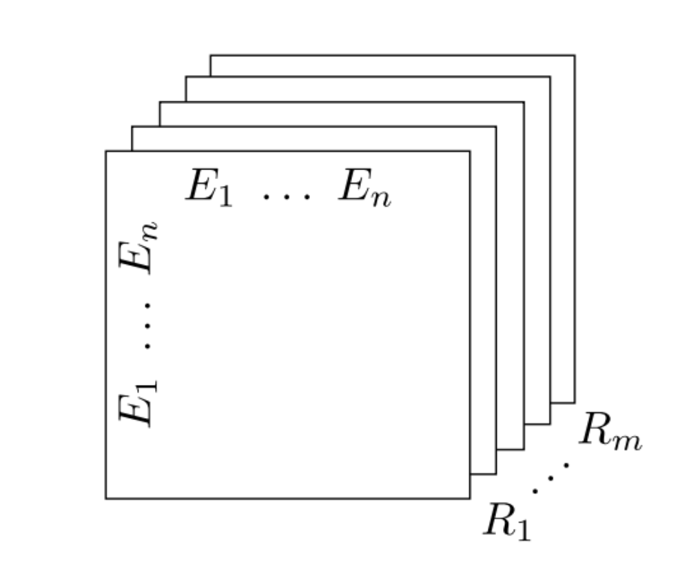
There are a couple of things to note about tensors representing RDF data. Entities in these tensors are not assumed to be homogeneous. Instead, they may instantiate different classes. Moreover, no distinction between ontological and instance relations is maintained, so that both classes and instances are modelled as entities. In this way, “ontologies are handled like soft constraints, meaning that the additional information present in an ontology guides the factorization to semantically more reasonable results” (Nickel et al. 2012, p. 273). Tensors representing RDF are usually very sparse due to high dimensionality and incompleteness, calling in for algorithms that leverage their sparseness for efficient execution, in particular for large data. Scalable processing of large RDF datasets in the tensor form is thus a challenge for optimization techniques. Interestingly, unlike RDF, tensors can represent n-ary relations without decomposing them into binary relations. What would in RDF require reification or named graphs can be captured with greater tensor order. This presents an opportunity for more expressive modelling outside of the boundaries of RDF.
We developed sparql-to-tensor, described in Section 6.2.9, to export RDF data from a SPARQL endpoint to the tensor form. The transformation is defined by SPARQL SELECT queries given to this export tool. Each query retrieves data for one or more RDF properties that constitute the relations in the output tensor. During the evaluation, we created and tested many tensors, each combining different properties and ways of pre-processing.
In most cases the retrieved relations corresponded to explicit RDF properties found in the source data. However, in a few select cases we constructed new relations. This was done either to avoid intermediate resources, such as tenders relating awarded bidders or proxy concepts relating unqualified CPV concepts, or to relate numeric values discretized to intervals. Since the original RESCAL algorithm does not support continuous variables, we discretized such variables via discretize-sparql, which is covered in Section 6.2.1.
Apart from binary numbers as tensor entries we used float numbers \(\mathcal{X}_{ijk} \in \mathbb{R} \colon 0 \leq \mathcal{X}_{ijk} \leq 1\) to distinguish the degrees of importance of relations. Float entries were used to de-emphasize less descriptive RDF properties, such as pc:additionalObject, or to model information loss from ageing, so that older contract awards bear less relevance than newer ones. We reused the ageing function from (Kuchař et al. 2016, p. 212) to compute the tensor entries:
\[\mathcal{A}(t_{0}) = \mathcal{A}(t_{x}) \cdot e^{-\lambda t}; t_{0} > t_{x}, t = t_{0} - t_{x}\]
In this function “\(\mathcal{A}(t_{0})\) is the amount of information at the time \(t_{0}\). \(\mathcal{A}(t_{x})\) is the amount of information at the time \(t_{x}\) when the information was created, \(\lambda\) is ageing/retention factor and \(t\) is the age of the information.” We assume \(\mathcal{A}(t_{x})\) to be equal to 1, the same value used for relations encoded without ageing. Since our dataset covers a period of 10 years, we use \(\lambda = 0.005\) that provides a distribution of values spanning approximately over this period. We used contract awards dates as values of \(t_{x}\) and the latest award date as \(t_{0}\). Award dates were unknown for the 2.3 % of contracts, for which we used the median value of the known award dates. The ageing function was implemented in a SPARQL SELECT query. Since the required natural exponential function is not natively supported in SPARQL, we used the extension function exp()89 built in the Virtuoso RDF store to compute it.
Instead of exporting all RDF data to the tensor format, we selected few features from it that we deemed to be the most informative. There are 76 different relations in the Czech public procurement dataset in total. Even more relations are available if we add the linked data. We experimented with selecting individual relations as well as their combinations to find out which ones produce the best results. We guided this search by the assumption that the contributions of the individual relations do not cancel one another out. Moreover, we ignore the possibility that features that do not bring improvement separately can produce improvement if used in combination, having synergic effect. Our heuristic for manual feature selection thus resembles simple hill-climbing.
2.7 Summary
Data preparation constituted a fundamental part of our research, since linked data offloads many concerns typically resolves on the application level to the data level. As a result of our data preparation effort a collection of interlinked datasets was created, as depicted in Fig. 6. The Czech public procurement dataset is central to this collection, including the primary data we used for matchmaking. The remaining datasets enrich the public procurement data with contextual information that can be turned into additional features for matchmaking. These datasets include the Common Procurement Vocabulary, three business registers mediated via the ARES system, Czech addresses dataset, NACE classification, and zIndex fairness scores. We encountered many challenges during the preparation of these datasets.
Since it is collectively created by thousands of officials representing contracting authorities over time, the Czech public procurement dataset suffers from the same problems as user-generated data, resulting in inconsistency and heterogeneity. Standardization can counteract these problems, but the standardization of public procurement data is imperfect at best. Moreover, as discussed in Section 1.5, public procurement is laden with disincentives to publishing good data. A key data quality problem we encountered was missing data. In particular, shared identifiers of entities involved in public procurement were non-existent, missing, or unreliable. In other cases there were conflicting values in the data, without enough annotations to discern the correct values and resolve their conflicts. A more detailed description of the quality of the Czech public procurement data is available in Soudek (2016a).
In order to combat the afore-mentioned data quality problems, we invested a lot of effort into linking (2.4) and fusion (2.5) of the data. The primary task we addressed was to reduce the variety of the data by conforming values, fusing aliases, or resolving value conflicts. Our approach to ETL adopted the separation of concerns as its basic design principle. In this way, we reduced the complexity of the data preparation and avoided bugs that could be caused by needless coupling. Moreover, the ETL procedures were specified in a declarative fashion, mostly by using XSLT and SPARQL Update operations, so that we could abstract from low-level implementation details that an imperative solution would need take into account. We made defensive data transformations with few assumptions about the processed data. The transformations usually checked if their input satisfied their assumptions and were able to cope with violations of the assumptions via fallback solutions. We designed a way of partitioning the transformations to allow scaling to larger data. We adopted the principles of content-based addressing for deduplication. Finally, when we could not remedy the problems of the data, we explicitly acknowledged the limitations of data, such as in case of the systemic biases manifest in public procurement data.
3 Matchmaking methods
We applied two methods to matching public contracts to bidders: case-based reasoning (CBR) and statistical relational learning (SRL). We first review what these methods have in common and then discuss their differences. Both methods learn from the same ground truth and have to cope with its limitations and biases, described in Section 3.1, such as having only positive training examples. In this ground truth, public contracts represent explicit demands and contract awards model past behaviour of bidders offering products or services. Both methods learn only from their input data, not from user feedback. In order to incorporate user feedback, it would need to be materialized as part of the input data. This approach is known as one-shot recommendation, and is typical for case-based recommenders in particular (Smyth 2007). We employed manual feature selection, corresponding to schema-aware matchmaking. Portability of the developed matchmakers is granted by the common data model underlain by the Public Contracts Ontology, which we covered in Section 2.1.1. The matchmakers therefore work with any dataset described by the PCO, such as the Czech public procurement dataset that constitutes our use case. Both methods are evaluated on the task of predicting the awarded bidders. The inverse task of recommending relevant public contracts to bidders is feasible as well, but we have not focused on it, since it mirrors the evaluated task.
The underlying technology we used to implement the matchmakers based on case-based reasoning, introduced in Section 1.6.1, is SPARQL (Harris and Seaborne 2013). Using the means of SPARQL we designed a custom-built matchmaking method, explained in detail in Section 3.2. In line with the CBR perspective, this method recasts data on awarded contracts as past cases to learn from. Viewed this way, awarded contracts can be considered as experiences of solved problems and contract awards can be thus interpreted as implicit positive ratings of the awarded bidders. Consequently, bidders awarded with most contracts similar to a given query contract can be recommended as potential awardees of the contract.
The developed matchmakers implement only the Retrieve and Reuse steps from the CBR cycle. The retrieved matches are ranked to produce recommendations for reuse. Including the Revise step would require the matchmakers to incorporate user feedback. The Retain step is not applicable if the proposed matches are not approved or disapproved in the Revise step. Both the Knowledge representation and the Problem formulation steps can be considered to be incorporated in data preparation, as documented in Section 2, since both cases and queries are materialized as data.
Matchmaking via SPARQL is conceived as a top-\(k\) recommendation task. It produces a list of bidders sorted by their degree to which they match the requirements of a given query contract. Since there is no explicit model built by this method, it is a case of lazy learning. Having no model to create up front allows to answer matchmaking queries in real time and to update the queried data in an incremental fashion.
Matchmakers based on statistical relational learning (SRL), which we presented in Section 1.6.2, are built on RESCAL (Nickel et al. 2011), In this case, we adopted an existing learning method for the matchmaking task, as explained in Section 3.3. Viewed from the perspective of SRL, matchmaking can be conceived as link prediction. In our setting, the task of matchmaking is predicting the most likely links between public contracts and their winning bidders.
Unlike the method based on SPARQL, RESCAL is a latent feature model. Since it builds a prediction model up front, it is an example of eager learning. Consequently, it operates in a batch mode that allows to update data only in bulk.
The key differences between the use of CBR and SRL for matchmaking are summarized in Table 1. Matchmaking can be also implemented via hybrid methods that combine multiple approaches. For instance, SPARQL can be used to pre-select matches and RESCAL can then re-rank this selection.
| Method | CBR | SRL |
|---|---|---|
| Underlying technology | SPARQL | RESCAL |
| Method origin | custom-built | reused |
| Learning method | lazy learning | eager learning |
| Matchmaking conceived as | top-\(k\) recommendation | link prediction |
| Features | observable | latent |
| Mode of operation | on demand query | batch |
| Update | incremental | bulk |
3.1 Ground truth
The fundamental part of the proposed matchmaking methods is the ground truth they are based on. We use past contracts awards as the ground truth from which the methods learn to assess matches. As such, it warrants a dedicated section to discuss its characteristics, in order to provide a better context for the following treatment of the matchmaking methods.
There are inherent downsides in our assumptions about the ground truth we used. The assumption that the awarded bidder is the best match for a contract is fundamentally problematic. We need to take into account that bidders may be awarded on the basis of adverse selection, e.g., caused by asymmetric distribution of information. Alternatively, tendering processes can suffer from collusion when multiple parties agree to limit open competition. In that case, rival bidders cooperate for mutual benefit, for instance, by bid rigging that involves submitting overpriced fake bids to make the real bids more appealing. Neither we can assume that bidders who were awarded multiple contracts from the same contracting authority have proven their quality. Instead, they may just be cases of clientelism.
Moreover, we have to rely on contract awards only, since we do not have explicit evaluations of the awarded bidders after finishing the contracts. Unfortunately, the lack of post-award data is common in public procurement:
“With a few exceptions such as Italy and Estonia, no government publishes information on contract implementation, making it impossible to know what happens after the contract is awarded — for example, did the suppliers deliver on time and budget?” (Mendes and Fazekas 2017)
Nor do we have any other relations between bidders and contracts in our dataset. Even though the profiles of contracting authorities link contracts with all bidders that submitted a valid bid, we have not included the profiles data in our dataset due to the effort involved in obtaining it.
We devised several counter-measures to ameliorate the impact of adverse selection in our ground truth. We experimented with discounting contract awards by the zIndex scores, described in Section 2.4.6.4, of their contracting authorities. However, this is a blunt tool, since it applies across the board for all contracts by a contracting authority. Within large contracting authorities each contract may be administered by a different civil servant, who may change over time.
We experimented with limiting our ground truth only to contracts awarded in open procedures. The intuition motivating this experiment is that a contract awarded in an open procedure enables fairer competition and thus avoids some risks of adverse selection.
We also considered restricting the contract awards to learn from by their award criteria. While it may seem that the simple criterion of lowest price is fair, it may be skewed by intentionally inflated fake bids due to bidder collusion. Other, more complex award criteria, such as those emphasizing qualitative aspects, can be problematic too. Their evaluation leaves more room for deliberation of contracting authorities, and as such, they can be made less transparent. Faced with this uncertainty, we ultimately avoided limiting our ground truth by contract award criteria.
Nevertheless, a likely outcome of these corrective measures is performance loss in the evaluation via retrospective data. Matchmakers may be underfitting, unable to sufficiently capture the underlying trends in the public procurement data, which too include the biases from adverse selection. On contrary, learning from all contract awards overfits, so that it includes the negative effects in public procurement as well. It may mistake random variability and systemic biases for causality. As a result, the inherent biases in our ground truth are difficult to account for.
3.2 SPARQL
The SPARQL-based matchmaker employs a case-based reasoning approach that learns from contracts awarded in the past. For each awarded contract a similarity to a given query contract is computed and the contracts are grouped by bidders who won them. The similarity scores in each group are aggregated and sorted in descending order. The matchmaker uses both semantic and statistical properties of data on which it operates. While the semantics of contract descriptions is employed in the similarity measurement, score aggregation reflects the statistics about the past participation of bidders in public procurement (Alvarez-Rodríguez et al. 2013, p. 122).
The initial version of the SPARQL-based matchmaker was introduced in (Mynarz et al. 2014). Our subsequent publication (Mynarz et al. 2015) covers an improved version of the matchmaker. The hereby described version is thus the third iteration of the matchmaker with extended configurability.
3.2.1 Benefits and drawbacks
This matchmaker explores the use of SPARQL (Harris and Seaborne 2013) for matchmaking. We introduced SPARQL in Section 1.4.2. The choice of this technology for matchmaking has both benefits and drawbacks.
3.2.1.1 Benefits of SPARQL for matchmaking
SPARQL is a native way of querying and manipulating RDF data. As it is designed for RDF, it is based on graph pattern matching. Graph patterns in SPARQL are based on data in the Turtle syntax (Beckett et al. 2014) extended with variables. Consequently, there is little impedance mismatch between data and queries, which improves developer productivity.
The design of SPARQL makes it into a universal tool for working with RDF. Thanks to its expressivity and declarative formulation it can be used for many varied tasks. For example, besides matchmaking we also adopted it as our primary tool for data preparation, as described in Section 2.
SPARQL is a standard (Harris and Seaborne 2013), so most RDF stores support it. The matchmaker can thus be set up simply by loading data into an RDF store. Since the matchmaker is limited to the standard SPARQL without proprietary add-ons or extension functions, it is portable across RDF stores compliant with the SPARQL specifications. As such it is not tied to any single RDF store vendor.
SPARQL operates directly on indices of RDF databases, so there is no need to pre-process data or build a machine learning model. In terms of recommender systems, we can consider it a memory-based approach. Thanks to this feature, SPARQL can answer matchmaking queries in real time. In particular, this is useful for recommendations from streaming data. Public procurement data shares some of the characteristics of streaming data as it becomes quickly obsolete due to its currency bound on fixed deadlines for tender submission.
3.2.1.2 Drawbacks of SPARQL for matchmaking
The benefits of SPARQL come with costs. As Maali (2014, p. 57) writes, the pure declarative nature and expressivity of SPARQL implies a high evaluation cost. RDF stores in general suffer from a performance penalty when compared to relational databases. Nevertheless, recent advancements in the application of the column store technology for RDF data brought on large performance improvements (Boncz et al. 2014, p. 23). SPARQL also lends itself to advanced query optimization that can avoid much of the performance costs.
In order to get the best performance of SPARQL, the matchmaker is limited to joins based on exact matches. SPARQL supports just exact matches natively. Exact matches can distinguish only between identical and non-identical resources. Fuzzy matches are needed to differentiate the degrees of similarity between resources. However, fuzzy matches have to be implemented on top of the default graph pattern matching in SPARQL. For example, the FILTER clauses can match partially overlapping strings or numbers within a given distance. SPARQL is not designed to perform such matches efficiently. Although SPARQL engines can optimize fuzzy matches, e.g., by using additional indices for literals, if literals are not indexed, they have to be analysed at query time, which incurs a significant performance penalty for queries employing fuzzy matches.
Performance of the matchmakers is also degraded by the unnecessary work SPARQL does for top-\(k\) queries. SPARQL employs the materialize-then-sort query execution scheme (Magliacane et al. 2012, p. 345), which implies that the matchmaker needs to compute scores for all matched solutions prior to sorting them, even though only top \(k\) matches are retrieved. Matchmaking in SPARQL depends on aggregations and sorting, both of which are examples of operations called the pipeline breakers in the query execution model. Such operations prevent lazy execution, since they require their complete input to be realized. For example, SPARQL treats sorting as a result modifier, which needs to be provided with all results.
3.2.2 Ranking matches
SPARQL queries retrieve exact matches satisfying the query conditions. Since SPARQL can tell only matches from non-matches, matches that satisfy the query partially are left out. Ranking of matches by the degree to which they satisfy the query thus needs to be implemented on top of SPARQL. Hence, we need to relax the match conditions to avoid filtering partial matches and then compute scores to rank the matches.
The matchmakers operate with a given query contract \(c_{q}\), which is matched to contracts from the set \(C\). They retrieve contract objects that overlap with the object of the query contract, which are optionally expanded to include related CPV concepts. Components of contract objects are weighted and these weights are combined into partial similarity scores. Partial similarities are then aggregated per bidder to produce the bidder’s match score.
3.2.2.1 Contract objects
Contract objects describe what products or services are sought by contracts. There are many ways how a contract object can be described. The matchmakers leverage contract objects described by terms from controlled vocabularies, such as CPV or the code list of contract kinds. Concretely, the matchmakers can use CPV concepts, either as main or additional objects or their qualifiers (pc:mainObject, pc:additionalObject), contract kinds (pc:kind), and service categories (isvz:serviceCategory). Accordingly, we define the set of properties \(P = \{\texttt{pc:mainObject}, \texttt{pc:additionalObject}, \texttt{pc:kind}, \texttt{isvz:serviceCategory}\}\) that associate concepts with contracts. The range of each of these properties is enumerated by a controlled vocabulary. We define the union of concepts in these vocabularies as \(Con = Con_{CPV} \cup Con_{kind} \cup Con_{\substack{service \\ category}}\). A concept can be either explicitly assigned to a contract or inferred via query expansion. To capture this distinction we use concept assignment \(ConA = \{\text{explicit}, \text{inferred}\}\). Contract object \(cobj\) is then a tuple \(((con, p), cona) \colon con \in Con, p \in P, cona \in ConA\), in which a concept \(con\) is paired with property \(p\) that associates the concept to a contract and this pair is qualified with the concept assignment \(cona\). Contract objects are represented as sets \(Cobj\) of these tuples. In order to obtain contract objects we use the function \(obj \colon C \cup \left\{c_{q}\right\} \to \mathbb{P}(Cobj)\). Here, \(\mathbb{P}(Cobj)\) denotes the power set of the set \(Cobj\). Accessing the elements of contract objects is in turn done by the function \(ccobj(cobj) = con \iff cobj = ((con, p), cona)\) for concepts and by the function \(pcobj(cobj) = p \iff cobj = ((con, p), cona)\) for properties.
3.2.2.2 Query expansion
Controlled vocabularies that describe contract objects can be semantically structured, such as via hierarchical or associative relations. Since relevance of a concept may entail relevance of concepts in its neighbourhood, we can leverage the structure of these vocabularies and perform expansion to include the related concepts in the query. In particular, we expand CPV concepts by following transitive hierarchical relations in this vocabulary. We follow either links to narrower concepts via skos:narrowerTransitive, links to broader concepts via skos:broaderTransitive, or links in both directions. Query expansion can be parameterized by the maximum number of hops followed to obtain a graph neighbourhood of the expanded concept. When a concept is expanded, its inferred concepts include those that are one to the maximum hops away from the expanded concept. Note that it is possible to infer a concept already included in the explicitly assigned concepts when these are hierarchically related. In such case, the concept appears twice in the contract object, distinguished by its concept assignment. Similarly, the same inferred concept can be reached more times by expanding different concepts. Such concept is present once in the results of query expansion since the results form a set. The figures 8 and 9 illustrate the query expansion, showing expansions to two-hop neighbourhoods.
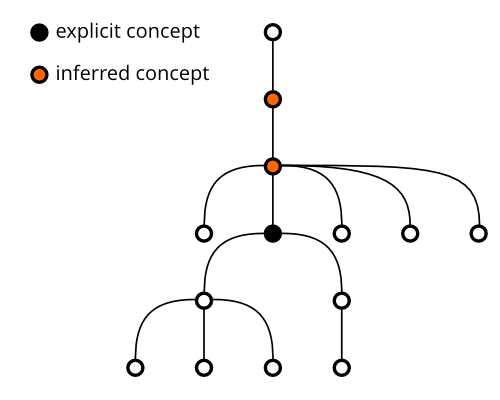
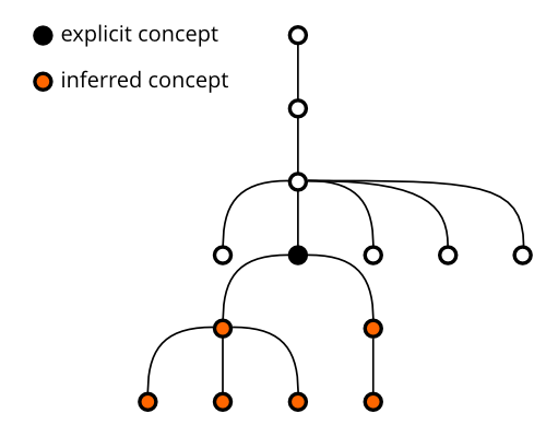
The arguments of the query expansion function \(exp\) are a set of contract objects, a direction of expansion, and a distance of the expansion. The direction of expansion \(Dir\) is the set \(\{\texttt{skos:broaderTransitive}, \texttt{skos:narrowerTransitive}\}\) indicating either the expansion to broader or narrower concepts. The distance is the maximum number of hops followed in the expansion. Consequently, the query expansion function can be defined as \(exp \colon \mathbb{P}(Cobj) \times Dir \times \mathbb{N}_{> 0} \to \mathbb{P}(Cobj)\). Bidirectional expansion of the set of contract objects \(\{cobj\} \subset Cobj\) to the distance \(dis\) can thus be computed as \(exp(\{cobj\}, \texttt{skos:broaderTransitive}, dis) \cup exp(\{cobj\}, \texttt{skos:narrowerTransitive}, dis)\). We only require \(exp\) to be monotonous, so that for every contract object \(cobj \in Cobj\) holds that \(((con, p), cona) \in cobj \;\; \Rightarrow \;\; ((con, p), cona) \in exp(cobj, dir, dis)\), and hence the function \(exp\) returns a union of its provided contract objects with the inferred contract objects. Concrete instantiations of \(exp\) can limit which input contract objects are expanded. In our case, either no contract objects are expanded or we only expand the explicitly assigned contract objects where \(p = \texttt{pc:mainObject}\) and \(con \in Con_{CPV}\).
3.2.2.3 Matching
The matchmakers examine only the exact matches between concepts of contract objects. Instead of matching complete contract descriptions or sets of concepts, matching on the finer level of individual concepts allows to capture partial overlaps between contracts. The predicate \(matches \colon Cobj \times Cobj \to \{T, F\}\) returns the boolean value true, denoted as \(T\), if concepts in the compared contract objects are the same, otherwise returning the boolean value false, denoted as \(F\).
\[matches(cobj_{a}, cobj_{b}) = \begin{cases} T & \text{if}\ ccobj(cobj_{a}) = ccobj(cobj_{b}) \\ F & \textrm{otherwise} \\ \end{cases}\]
Here, \(ccobj(cobj_{a})\) accesses the concept in the contract object \(cobj_{a}\). As is evident, in order to achieve a match, the ranges of the properties in the compared contract objects must be the same.
Matching considers its input as the query contract, while the other contracts are treated as potential matches. The function \(match \colon \left\{c_{q}\right\} \times Dir \times \mathbb{N}_{> 0} \to \mathbb{P}(CMA)\) retrieves concept-mediated associations matching a given query contract \(c_{q}\).
\[match(c_{q}, dir, dis) = \bigcup \left\{ \begin{split} & (ccobj(o_{q}), pcobj(o_{q}), pcobj(o_{m}), c_{m}) \colon \\ & o_{q} \in exp(obj(c_{q}), dir, dis), \\ & c_{m} \in C, \\ & o_{m} \in obj(c_{m}), \\ & matches(o_{q}, o_{m}) \end{split}\right\}\]
The direction of expansion \(dir\) and the distance \(dis\) are passed as arguments to the query expansion function \(exp\). The function \(match\) produces a set of concept-mediated associations \(CMA\) that are defined as 4-tuples \((con, p_{q}, p_{m}, c_{m}) \colon con \in Con, p_{q} \in P, p_{m} \in P, c_{m} \in C\). We call them concept-mediated associations since they connect the query contract with the matched contracts via concepts. In each association \(p_{q}\) is a property associating a concept \(con\) to the query contract and \(p_{m}\) is a property associating \(con\) to a matched contract \(c_{m}\).
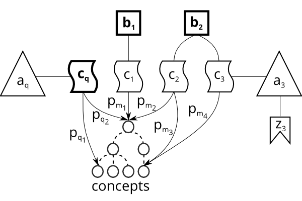
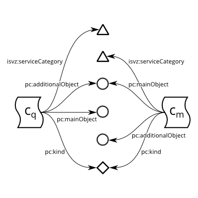
Fig. 10 shows an overall diagram of concept-mediated associations. The query contract \(c_{q}\) is associated to the matched contracts \(c_{1}, c_{2}, c_{3} \in C\) via concepts that are assigned to the query contract via \(p_{q_{i}}\) and to the matched contracts via \(p_{m_{i}}\). As shown in Fig. 11, contracts may be associated through different kinds of concepts. The matched contracts in turn lead to bidders \(b_{1}, b_{2} \in B\). Here, \(B\) is the set of known bidders. Contracting authority of \(c_{q}\) is marked as \(a_{q}\), while the contracting authority of \(c_{3}\) is denoted as \(a_{3}\). For \(a_{3}\) a zIndex score \(z_{3}\) is available.
3.2.2.4 Weighting
The matchmaker can translate each part of concept-mediated associations into a weight \(w \in \mathbb{R} \colon 0 \leq w \leq 1\). In certain variants of the matchmakers the reference to concept \(con\) is transformed to an inverse document frequency (IDF), in particular when dealing with concepts obtained via query expansion. Similarly, the properties \(p_{q}\) and \(p_{m}\) can be weighted according to the degree in which they contribute to the similarity between contracts. Likewise, the contract \(c_{m}\) can be turned into a weight corresponding to its contracting authority’s fairness score. Some weights are given by data, such as the fairness scores, or derived from it, such as IDFs. Others can be provided as configuration of the matchmaker, such as the inhibiting weight of pc:additionalObject.
There are several concrete ways in which weights can be applied to CPV concepts. The matchmaker may apply an inhibiting weight to de-emphasize the concepts associated with contracts via the pc:additionalObject property in contrast to the pc:mainObject. These weights are applied both to \(p_{q}\) and \(p_{m}\). Similarly, qualifying concepts from the CPV’s supplementary vocabulary can be discounted via a lower weight. Concepts inferred by query expansion can be weighted either by a fixed inhibiting weight or their IDF.
Inverse document frequency is used to reduce the impact of popular CPV concepts on matchmaking. Unlike infrequent and specific concepts, the popular ones may have lesser discriminative power to determine the relevance of contracts described by them. Raw IDF of CPV concepts is defined as \(idf \colon Con_{CPV} \to \mathbb{R}^{+}\) and is computed as follows:
\[idf(con) = \log\frac{\left\vert{C}\right\vert}{1 + \left\vert{\{c \in C \colon ((con, p), cona) \in obj(c)}\right\vert}\]
The denominator in the formula is incremented by 1 to avoid division by zero in case of concepts unused in contract objects. Subsequently, we normalize IDF into the range of \(\left[0, 1\right]\) by using its maximum value in order to be able to use it as a weight.
\[idf'(con) = \frac{idf(con)}{max(\{con' \in Con_{CPV} \colon idf(con')\})}\]
Besides CPV, weights can be applied to specific properties from \(P\). In particular, the matchmaker can inhibit the objects of pc:kind when used in combination with CPV. This property indicates the kinds of contracts, such as works or supplies, which classify contracts into broad categories.
The matchmaker also allows to weight the matched contracts indirectly via weights of their contracting authorities. We use zIndex scores as weights of contracting authorities. These scores are taken from the dataset covered in Section 2.4.6.4. We assume the function \(authority \colon C \to Auth\) returns the contracting authority of a given contract. Here, \(Auth\) denotes the set of known contracting authorities. The function \(zindex \colon Auth \to \left[0, 1\right]\) produces a weight given to a contracting authority by the zIndex score. The function weighting by zIndex can then be defined by composing these functions; i.e. \(zindex \circ authority\).
3.2.2.5 Aggregation functions
We use aggregation functions to turn weights into match scores. Weights of components in each concept-mediated association are combined using the function \(comb\). The combined weights are aggregated via the function \(agg\).
Aggregation functions take multiple numeric inputs and combine them into a single output. The matchmaker uses these functions to combine weights and partial similarity scores to form a match score. As such, aggregation functions constitute an important part of ranking. In terms of fuzzy logic, aggregation functions can be interpreted as generalizations of logical conjunction and disjunction. Instead of only boolean values, their inputs can be treated as degrees of probability, where 0 indicates impossibility and 1 indicates certainty. Aggregation function \(f\) can thus be defined as \(f \colon \left[0, 1\right] \times \left[0, 1\right] \to \left[0, 1\right]\) (Beliakov et al. 2015, p. 785).
The typical examples of these functions are triangular norms (t-norms) and conorms (t-conorms). T-norms generalize conjunction and t-conorms generalize disjunction. The basic t-norms can be defined as follows (Beliakov et al. 2015, p. 792):
- Gödel’s t-norm (minimum t-norm): \(T_{min}(x, y) = min(x, y)\)
- Product t-norm: \(T_{P}(x, y) = x \cdot y\)
- Łukasiewicz’s t-norm: \(T_{L}(x, y) = max(x + y - 1, 0)\)
We use these t-norms to combine weights by the function \(comb\). The basic t-conorms, complementary to the mentioned t-norms, are the following:
- Gödel’s t-conorm (maximum t-conorm): \(S_{max}(x, y) = max(x, y)\)
- Product t-conorm (probabilistic sum): \(S_{P}(x, y) = x + y - x \cdot y\)
- Łukasiewicz’s t-conorm (bounded sum): \(S_{L}(x, y) = min(x + y, 1)\)
We use these t-conorms to aggregate contract similarities into the match scores of bidders by the function \(agg\). Both t-norms and t-conorms are associative and commutative, so their computation can be extended to arbitrary collections of weights.
Given these formulas we can summarize how the matchmaker works. The matchmaker retrieves concept-mediated associations \(cma \in match(c_{q}, dir, dis)\) for a query contract \(c_{q}\) using a configuration of query expansion and weighting. Concept associations are partitioned into subsets by the bidder awarded with the contract \(c_{m}\) from the association. Each concept-mediated association in these partitions is subsequently weighted to produce an n-tuple of weights. The obtained weights are combined to a single weight of each concept-mediated association via the \(comb\) function. An n-tuple of the combined weights from a partition by bidder can be then aggregated by the \(agg\) function to produce match scores. Finally, the matches are sorted by their score in descending order and the top-\(k\) matches are output.
3.2.3 Blind matchmakers
Apart from the above-described matchmakers, we also implemented three blind approaches for matchmaking, none of which considers the query contract. The most basic is the random matchmaker that recommends bidders at random. While it is hardly going to deliver a competitive accuracy, it produces diverse results. An approach contrary to random matchmaking is the recommendation of the top-most popular bidders. For each contract this matchmaker recommends the same bidders that were awarded the most contracts. A similar approach is employed in the matchmaker that recommends bidders with the highest score computed by the PageRank-like algorithm implemented by the Virtuoso-specific IRI_RANK (OpenLink Software 2017). Since this score uses a proprietary extension of SPARQL, it is an exception from our constraint to standard SPARQL. These conceptually and computationally simpler approaches are used as baselines to which we can contrast the more sophisticated approaches in evaluation.
3.2.4 Implementation of SPARQL-based matchmakers
The matchmakers are implemented by SPARQL query templates. Each template receives a configuration and produces a SPARQL query. The generated queries are executed on the configured SPARQL endpoint and return ordered sets of matches. Each kind of matchmaker corresponds to a particular query template. It may also expose specific parameters that can be provided via the configuration.
The basic graph pattern considered in most matchmakers is illustrated in Listing 3 using the SPARQL 1.1 Property Path syntax. The path is complicated by intermediate resources proxying CPV concepts connected via skos:closeMatch, as described in Section 2.1.2.
Listing 3: Matchmaker's basic SPARQL property path
?queryContract ^pc:lot/pc:mainObject/skos:closeMatch/
                         ^skos:closeMatch/^pc:mainObject/pc:lot/
                         pc:awardedTender/pc:bidder ?matchedBidder .
Apart from our baseline matchmaker, which uses the property path in Listing 3, the implementation of the matchmakers is based on nested sub-queries and VALUES clauses used to associate the considered properties with weights.
We implemented query expansion via SPARQL 1.1 property paths. Property paths allow us to retrieve concepts reachable within a given maximum number of hops transitively following the hierarchical relations in CPV. We use the short-hand notation {1, max} for these property paths. It defines a graph neighbourhood at most max hops away. This notation is not a part of the SPARQL standard, but it is formally defined by Seaborne (2014), and several RDF stores, including Virtuoso, support it. However, it can be rewritten to the more verbose standard SPARQL notation if full standards-compliance is required.
Score aggregation via aggregation functions is done using SPARQL 1.1 aggregates. However, probabilistic sum requires aggregation by multiplication, which cannot be implemented directly in SPARQL since it lacks an operator to multiply grouped bindings. Therefore, we implemented this aggregation function via post-processing of SPARQL results. Eventually, since the difference on the evaluated metrics between probabilistic sum and summation (\(a + b\)) turned out to be statistically insignificant, we opted for summation, which can be computed directly in SPARQL and is marginally faster. A side effect of this implementation is that the match scores in the matchmakers using this aggregation function are not normalized.
The execution time of the matchmakers can be improved by common optimization techniques for SPARQL. We reordered triple patterns in the matchmaking queries in order to minimize the cardinalities of the intermediate results. We reduced unnecessary intermediate bindings via blank nodes and property paths. Performance can be also enhanced by storing pre-computed data. While there is no need for data pre-processing specific for the matchmakers, derived data that changes infrequently can be materialized and stored in RDF. Doing so can improve the performance of matchmakers by avoiding the need to recompute the derived data at query time. This benefit is offset by increased use of storage space and an additional overhead with updates, since materialized data has to be recomputed when the data it is derived from changes. We used materialization for pre-computing IDF of CPV concepts. While IDF can be computed on the fly, we decided to pre-compute it and store it as RDF. Computation of IDF is implemented via two declarative SPARQL Update operations, the first of which uses a Virtuoso-specific extension function for logarithm (bif:log10()), and the second normalizes the IDFs using the maximum IDF.
The implementation of the matchmakers, described in Section 6.2.4, is built as a wrapper over the Virtuoso RDF store. Example SPARQL queries used by the matchmakers can be found at https://github.com/opendatacz/matchmaker/wiki/SPARQL-query-examples.
3.3 Tensor factorization
Tensor factorization is a method for decomposing tensors, which are described in Section 2.6.2, into lower-rank approximations. The rank of a tensor \(\mathcal{X}\) is “the smallest number of rank one tensors that generate \(\mathcal{X}\) as their sum” (Kolda and Bader 2009). \(\mathcal{X}\) is an \(N\)th order rank one tensor when it “can be written as the outer product of \(N\) vectors” (Kolda and Bader 2009): \(\mathcal{X} = \mathbf{a}^{(1)} \circ \mathbf{a}^{(2)} \circ \cdots \circ \mathbf{a}^{(N)}\). Determining the tensor’s rank is known to be an NP-hard problem (Sidiropoulos et al. 2017), so in practice low-rank approximations are used instead. As such, tensor factorization can be considered a dimensionality reduction technique based on the assumption that there exists a low-dimensional embedding of the entities in tensors. In fact, computing a tensor factorization is possible because most tensors exhibit latent structure. A theoretical generalization of the abilities of tensor factorization is provided in Nickel and Tresp (2013a).
Tensor factorization can be regarded as a generalization of matrix factorization for higher-dimensional arrays. Unlike matrices, tensor representation offers a greater fidelity, since it can preserve the structure of higher order relations that would be otherwise lost were these relations collapsed into a matrix representation (Mørup 2011). Tensor factorization is also referred to as tensor decomposition. Here, for clarity, we use tensor factorization to denote the process of computing its product, the tensor decomposition.
Statistical relational learning, introduced in Section 1.6.2, employs tensor factorization for link prediction. Viewed from this perspective, the input of factorization is considered to be a noisy, partially observed tensor. Tensor decomposition produced by the factorization can be in turn used to reconstruct an approximation of the complete tensor. In this way, we can use tensor decompositions as prediction models that explain the predicted links by latent features of entities. Tensor factorization typically yields good results for link prediction in domains characterized by high dimensionality, sparseness (Nickel et al. 2011), and noise (Zhiltsov and Agichtein 2013, p. 1254). So far, it has found applications in many domains, including chemometrics or social network mining. There were also a few attempts applying tensor factorization to RDF, such as TripleRank (Franz et al. 2009), the dominant one being RESCAL (Nickel et al. 2011). We reused RESCAL for matchmaking via tensor factorization.
3.3.1 RESCAL
RESCAL is a machine learning algorithm for factorization of third-order tensors. It factorizes a tensor \(\mathcal{X}\) with \(n\) entities to a rank-\(r\) representation, so that each frontal slice \(\mathcal{X}_{k}\) of the tensor can be approximately reconstructed via matrix product from the decomposition to latent components, as shown in Fig. 12, using this formula:
\[X_{k} \approx AR_{k}A^{T}\qquad(1)\]
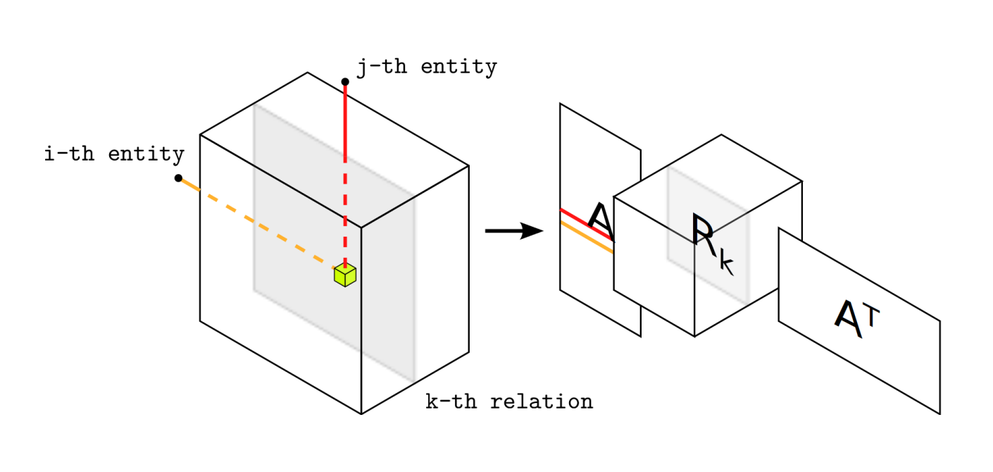
In this formula, \(A\) is an \(n \times r\) matrix containing the latent component representation of entities in \(\mathcal{X}\), \(A^{T}\) is its transposition, and \(R_{k}\) is a square \(r \times r\) matrix that models the interactions of the latent components in the \(k\)th predicate (Nickel et al. 2011). Using this decomposition, RESCAL “explains triples via pairwise interactions of latent features” (Nickel et al. 2016, p. 17). Unlike in other latent feature models, the latent variables in RESCAL do not describe entity classes but latent entity factors instead (Tresp and Nickel 2014). The rank \(r\) is a “central parameter of factorization methods that determines generalization ability as well as scalability” (Nickel et al. 2014). While higher \(r\) increases the expressiveness of the latent features, it also increases the runtime of tensor factorization as well as its propensity for overfitting. Consequently, setting \(r\) to an appropriate value is a key trade-off to be made when tuning RESCAL.
RESCAL uses distinct latent representations of entities as subjects and objects, which enables efficient information propagation to capture correlations over long-range relational chains (Nickel and Tresp 2013b, p. 619) that may span heterogeneous relations. In this way, RESCAL is able to leverage contextual data that is more distant in the relational graph for collective learning, which we described in Section 1.6.2. Unlike other factorization methods that cannot model collective learning sufficiently, “the main advantage of RESCAL, […] is that it can exploit a collective learning effect when applied to relational data” (Nickel et al. 2012, p. 272).
RESCAL achieves a leading performance for link prediction tasks. It was shown to be superior for link prediction tasks on several datasets. Moreover, it scales better to large data than many traditional methods for statistical relational learning, such as Markov logic networks. Nickel et al. (2012) demonstrated how the execution of RESCAL can be parallelized and distributed across multiple computing nodes. RESCAL is also fundamentally simpler than other tensor factorization methods. Unlike similar algorithms, RESCAL stands out by a low Kolmogorov complexity. It is implemented only in 120 lines of code in Python (Nickel et al. 2011) using solely the NumPy90 library.
Many extensions of RESCAL were proposed. Its state-of-the-art results and conceptual simplicity invite improvements. The aspects that the extensions deal with include negative training examples, handling literals, or type constraints.
RESCAL adopts the local closed world assumption (LCWA), which is used often for training relational models (Nickel et al. 2016, p. 13). It “approaches the problem of learning from positive examples only, by assuming that missing triples are very likely not true, an approach that makes sense in a high-dimensional but sparse domain” (Nickel et al. 2012, p. 273). However, “training on all-positive data is tricky, because the model might easily over generalize” (Nickel et al. 2016, p. 24). In order to avoid underfitting, negative examples can be generated via type constraints for predicates or valid ranges of literals. Nickel et al. (2016) propose generating negative examples by perturbing true triples. For instance, switching subjects in triples sharing the same functional property produces false, but type-consistent triples.
The original version of RESCAL (Nickel et al. 2011) uses only object properties as relations. Datatype properties with literal objects can only be used if the literals are treated as entities. When literals are included as entities in a tensor, although they never appear as subjects, the tensor’s sparseness grows. Moreover, since the number of distinct literals may significantly surpass the number of entities, this naïve treatment will greatly expand the dimensionality of the input tensor. Both high dimensionality and sparseness thereby increase the complexity of computing the factorization. Minor improvements can be attained by pre-processing literals, such as by discretizing numeric values, tokenizing plain texts, and stemming the generated tokens. Nevertheless, treatment of literals warrants a more sophisticated approach. To address this issue, Nickel et al. (2012) introduced an extension of RESCAL to handle literals via an attribute matrix that is factorized conjointly with the tensor with relations between entities. In a similar vein, Zhiltsov and Agichtein (2013) proposed Ext-RESCAL, an approach using term-based entity descriptions that include names, other datatype properties as attributes, and outgoing links.
Several researchers (Chang et al. (2014), Krompaß et al. (2014), Krompaß et al. (2015)) investigated adding type constraints to RESCAL. These constraints improve RESCAL by preventing type-incompatible predictions. The type compatibility can be determined by interpreting the rdfs:domain and rdfs:range axioms under LCWA or by evaluating custom restrictions, such as requiring the subject entity to be older than the object entity when predicting parents. These type constraints can be represented as binary matrices (Krompaß et al. 2014) indicating compatibility of entities. The original RESCAL considers all entities for possible relations, notwithstanding their type, which increases its model complexity and leads to “an avoidable high runtime and memory consumption” (Krompaß et al. 2014). Even though RESCAL is faster than the type-constrained approach with the same rank, using type constraints typically requires a lower rank to produce results that RESCAL is able of achieving only at higher ranks.
Other notable extensions of RESCAL add time awareness or tensor slice similarities. Kuchař et al. (2016) enhanced link prediction via RESCAL to be time-aware. We used this approach in data pre-processing, as described in Section 2.6.2, to model decaying relevance of older contract awards. Padia et al. (2016) obtained better results from RESCAL by considering the similarities of tensor slices.
3.3.2 Ranking matches
We applied link prediction via RESCAL to matchmaking, assuming that the tensor decomposition produced by RESCAL can accurately model the affinities between contracts and bidders. Probabilities of links predicted in the tensor slice representing contract awards can be obtained by reconstructing the slice from the tensor decomposition. Given the slice \(R_{award}\) for contract awards from the latent factor tensor \(\mathcal{R}\) produced by RESCAL, we can obtain predictions of entities awarded with the contract \(c\) by following Eq. 1 and computing the predictions vector \(p = A_{c}R_{award}A^{T}\). Entries in \(p\) can be interpreted as probabilities of the contract \(c\) being awarded to entities at corresponding indices in \(p\). Using the indices of bidders we can filter the entries in \(p\) and then rank them in descending order to obtain the best matches for \(c\).
We used no minimal threshold to filter out irrelevant matches. As reported in (Nickel et al. 2012), determining a reasonable threshold is difficult, because the high sparseness of the input tensors causes a strong bias towards zero (Nickel et al. 2012, p. 274). Consequently, instead of setting an arbitrary threshold, we ranked the predictions by their probability and projected the top-ranking predictions as the matches. This decision is a trade-off erring on the side of delivering less relevant results instead of producing fewer or no results.
Unlike SPARQL, RESCAL is a batch approach that cannot produce results in real time. First, it needs to factorize the input tensor to a decomposition that models the tensor. Once this model is built, predictions for individual contracts can be computed on demand. RESCAL is hence slow to cope with changing data. Matchmaking via RESCAL is thus more appropriate if the matches are delivered via periodic subscriptions instead of on-demand queries.
3.3.3 Implementation of RESCAL-based matchmakers
We implemented matchmaker-rescal, described in Section 6.2.5, a thin wrapper of RESCAL that runs our evaluation protocol, explained in Section 4.2. Instead of extending RESCAL, our contribution lies in the data preparation and pre-processing described in Section 2.6.2.
When developing the RESCAL wrapper, we needed to take several aspects of performance into consideration. Due to the size of the processed data it is important to leverage its sparseness, which is why we employ efficient data structures for sparse matrices from the SciPy91 library. Due to its size in memory, reconstructing the whole predictions slice is unfeasible for larger datasets. In order to reduce the memory footprint of the RESCAL-based matchmakers, we avoided reconstructing the whole predictions slice from the RESCAL factorization, but computed only the top-\(k\) results instead. Predictions were computed for each row separately, so that the rows could be garbage-collected to free memory. In order to enable parallelization, it was important to compile the underlying NumPy library with the OpenBLAS92 back-end, which allows to leverage multi-core machines for parallel computation of low-level array operations, such as the matrix product that is central to RESCAL.
4 Evaluation
We attempted to demonstrate the utility of the developed matchmakers by evaluating several metrics. We chose metrics that approximate the accuracy and diversity of matchmaking. The metrics were evaluated in an offline setup.
Offline evaluation is an experimental setting in which past interactions are used as ground truth. In this setting, some interactions are withheld and the evaluated system is assessed on its ability to fill in the missing interactions. Offline evaluation is defined in the recommender systems research in contrast to online evaluation. While online evaluation involves users in real-time, offline evaluation approximates actual user behaviour by using pre-recorded user interactions. Offline evaluation then “consists of running several algorithms on the same datasets of user interactions (e.g., ratings) and comparing their performance” (Ricci et al. 2011, p. 16).
While using historical user interaction data for evaluation is a common practice (Jannach et al. 2010, p. 169), it has several flaws that reduce its predictive power. In addition to the domain-specific limitations of the ground truth, which we described in Section 3.1, the datasets used for offline evaluation can be incomplete and may contain systemic biases. Ground truth in the datasets is incomplete, since it typically contains only a fraction of true positives. In most cases, users review only few possible matches, excluding the rest, notwithstanding its relevance, from the true positives. Consequently, if the evaluated system recommends relevant items that are not in the ground truth, these matches are ignored. In other words, “when incomplete datasets are used as ground-truth, recommender systems are evaluated based on how well they can calculate an incomplete ground-truth” (Beel et al. 2013, p. 11).
Due to these limitations offline evaluation has a weak prediction power. As such, “offline evaluations of accuracy are not always meaningful for predicting the relative performance of different techniques” (Garcin et al. 2014, p. 176). Offline evaluation can tell which of the evaluated approaches provides better results, but it cannot tell if an approach is useful. There is a limited correspondence between the evaluated metrics and usefulness in the real world. Whether an approach is useful can be evaluated only by real users. This is what online evaluation or qualitative evaluation can help with.
However, one can also argue that “offline evaluations are based on more thorough assessments than online evaluations” (Beel et al. 2013). Ground truth in offline evaluation may be derived from more thorough examination of items, involving multiple features in tandem, while online evaluation may rely on superficial assessment, such as click-throughs based on titles only.
Online evaluation is commonly recommended as a remedy to the afore-mentioned limitations of offline evaluation. As a matter of fact, results of online evaluation can differ widely from the results of offline evaluation. Several studies found that the “results of offline and online evaluations often contradict each other” (Beel et al. 2013, p. 7) or acknowledged that “there remains a discrepancy in the offline evaluation protocols, and the online deployment and accuracy estimate of the algorithms in a real-life setting” (Said et al. 2013). However, conducting online evaluation is expensive since it requires an application with real users. In order to attract a sufficient mass of users to make the findings from the evaluation statistically significant, the application must be relatively mature and proven useful. Moreover, we wanted to explore a large space of different matchmaker configurations, for which carrying out online evaluation would be prohibitively expensive. Ultimately, due to the large effort involved in setting up online evaluation we restricted our work to offline evaluation.
We used offline evaluation to filter matchmaking methods and configurations to find the most promising ones. Since we test different matchmakers in the same context, this evaluation can be also considered a trade-off analysis (Wieringa 2014, p. 260), in which we balance the differences in the evaluated measures.
4.1 Ground truth
We conducted offline evaluation using retrospective data about awarded public contracts. As we described previously in Section 3.1, the ground truth poses several challenges and limitations that the matchmakers have to deal with. Matchmaking was tested on the task of predicting the awarded bidder. In our case, we treat contract awards as explicit positive user feedback. Thus, in terms of (Beel et al. 2013), we use a “user-offline-dataset”, since it contains implicit ratings inferred from contract awards.
Due to the design of the chosen evaluation task, we had to adjust our ground truth data. Since we evaluate matchmaking as a prediction of the awarded bidders, we need each public contract to have a single winner. However, that is not the case for around 1 % of the public contracts in our dataset. This may be either in error or caused by members of the winning groups of bidders being listed separately. For example, framework agreements may be awarded to multiple bidders. For the sake of simplicity we decided to exclude these contracts from our ground truth.
4.2 Evaluation protocol
Our evaluation protocol is based on n-fold cross-validation. We split the evaluation data into training and testing dataset. The testing dataset contains the withheld contract awards that a matchmaker attempts to predict. We used 5-fold cross-validation, so that we divided the evaluation data into five non-overlapping folds, each of which was used as a testing dataset, while the remaining folds were used for training the evaluated matchmakers. In this way we tested prediction of each contract award in the ground truth.
When evaluating matchmakers that take time into account, we split the ground truth so that the training data precedes the testing data. First, we sort the ground truth by contract award date in ascending order. If the award date is unknown, we use its median value. The sorted ground truth is then split in five folds. The second or later folds are consecutively used as the testing data, while all the previous folds constitute the training data. The first fold is therefore never used for testing, so we test only four folds. In this way we avoid training on data from the future relative to the tested data.
4.3 Evaluated metrics
The objectives we focus on in offline evaluation are accuracy and diversity of the matchmaking results. The adopted evaluation metrics thus go beyond those that reflect accuracy. While we aim to maximize the metrics of accuracy, in case of the non-accuracy metrics, we strive to increase them without degrading the accuracy.
We define the evaluation metrics using the following notation. Let \(C\) be the set of public contracts and \(B\) the set of bidders who were awarded at least one contract. The function \(\mathit{match10}_{m}\colon C \to \mathbb{P}(B)\), where \(\mathbb{P}(B)\) is the powerset of \(B\), returns an ordered set of 10 best-matching bidders recommended by matchmaker \(m\) for a given public contract. We considered only the first 10 results due to the primacy effect, which describes that users analyze the items at the beginning of a recommendation list more frequently.93 The function \(winner\colon C \to B\) returns the winning bidder to whom a contract was awarded. The function \(wrank\colon C \to \mathbb{N}_{> 0} \cup \{ \text{nil} \}\) gives the rank of the bidder who won a given public contract.
\[wrank(c) = \small \begin{cases} n \colon winner(c)\, \textrm{is in position}\, n\, \textrm{in}\, \mathit{match10}_{m}(c) & \text{if}\ winner(c) \in \mathit{match10}_{m}(c) \\ \quad\textrm{nil} & \textrm{otherwise} \\ \end{cases} \normalsize\]
The function \(awards\colon B \to \mathbb{N}\) returns the number of contracts awarded to a given bidder.
\[awards(b) = \left\vert{c \in C : winner(c) = b}\right\vert\]
We measured accuracy using hit rate at 10 (HR@10) and mean reciprocal rank at 10 (MRR@10). HR@10 (Deshpande and Karypis 2004, p. 159) is the share of queries for which hits are found in the top 10 results. We consider hits to be the results that include the awarded bidder. We adopted HR@10 as the primary metric that we aim to increase. This metric can be calculated for the matchmaker \(m\) as follows:
\[HR@10 = \frac{\left\vert{c \in C : winner(c) \in \mathit{match10}_{m}(c)}\right\vert}{\left\vert{C}\right\vert}\]
MRR@10 (Craswell 2009) is the arithmetic mean of multiplicative inverse ranks. Multiplicative inverse rank \(mir\colon C \to \mathbb{Q}_{> 0}\) for matchmaker \(m\) can be defined as such:
\[mir(c)=\begin{cases} \frac{1}{wrank(c)} & \text{if}\ winner(c) \in \mathit{match10}_{m}(c) \\ 0 & \text{nil} \end{cases}\]
This metric is used for evaluating systems where “the user wishes to see one relevant document” (Craswell 2009) and it is “equivalent to Mean Average Precision in cases where each query has precisely one relevant document” (Craswell 2009). This makes it suitable for our evaluation setup, since for each query (i.e. a contract) we know only one true positive (i.e. the awarded bidder). MRR@10 reflects how prominent the position of the hit is in the matchmaking results. We aim to increase MRR@10, corresponding to a lower rank the hit has. MRR@10 can be defined as follows:
\[MRR@10 = \frac{1}{\left\vert{C}\right\vert}\sum_{c \in C} mir(c)\]
The adopted metrics that go beyond accuracy include prediction coverage (PC), catalog coverage at 10 (CC@10), and long-tail percentage at 10 (LTP@10). PC (Herlocker et al. 2004, p. 40) measures the amount of items for which the evaluated system is able to produce recommendations. We strive to increase PC to achieve a near-complete coverage. PC for the matchmaker \(m\) is defined as the share of the queries for which non-empty results are returned.
\[PC = \frac{\left\vert{c \in C : \mathit{match10}_{m}(c) \neq \varnothing}\right\vert}{\left\vert{C}\right\vert}\]
CC@10 (Ge et al. 2010, p. 258) reflects diversity of the recommended items. Systems that recommend a limited set of items have a low catalog coverage, while systems that recommend many diverse items achieve a higher catalog coverage. We compute CC@10 for the matchmaker \(m\) as the number of distinct bidders in the top 10 results for all contracts divided by the number of all bidders.
\[CC@10 = \frac{\left\vert{\bigcup_{c \in C} \mathit{match10}_{m}(c)}\right\vert}{\left\vert{B}\right\vert}\]
LTP@10 (Adomavicius and Kwon 2012) is a metric of novelty, which is based on the distribution of the recommended items. Concretely, it measures the share of items from the long tail in the matchmaking results. If we sort bidders in descending order by the number of contracts awarded to them, the first bidders that account for 20 % of contract awards form the short head and the remaining ones constitute the long tail. In case of the Czech public procurement data, 20 % of the awarded contracts concentrates among the 101 most popular bidders from the total of 14388 bidders in the dataset. To avoid awarding contracts only to a few highly successful bidders, we aim to increase the proportion of recommendations from the long tail of bidders. Let \((b_{1}, \dots, b_{n})\) be a list of all bidders \(b_{i} \in B\), so that \((i \prec j) \implies awards(b_{i}) \geq awards(b_{j})\) and the bidders are sorted in descending order by the number of contracts awarded to them. The short head \(SH\) of this ordered list can be then defined as:
\[SH = (b_{1},\dots,b_{e});\quad \textrm{so that}\, e : \sum_{k = 1}^{e - 1} awards(b_{k}) < \frac{\left\vert{C}\right\vert}{5} \leq \sum_{l = 1}^{e} awards(b_{l})\]
The formula defines \(SH\) as delimited by the index \(e\) of the bidder with the awards of whom the short head accumulates the 20 % of all awarded contracts (i.e. \(\frac{\left\vert{C}\right\vert}{5}\)). Long tail \(LT\) is the complement of the short head (\(LT = B \setminus SH\)). We then calculate LTP@10 for the matchmaker \(m\) as follows:
\[LTP@10 = \frac{\sum_{c \in C} \left\vert{\mathit{match10}_{m}(c) \cap LT}\right\vert}{\sum_{c \in C} \left\vert{\mathit{match10}_{m}(c)}\right\vert}\]
Due to our evaluation setup we avoided some of the usual metrics from information retrieval in general and from recommender systems in particular. Both precision and recall have limited use in our case, since only one true positive is known. If we consider top 10 results only, the precision would be either 1/10 or 0, while the recall would be either 1 or 0. This problem is known as class imbalance (Christen 2012). Results with the status of non-match are much more prevalent in matchmaking than those with the status of match, which skews the evaluation measures that take non-matches into account.
The rest of this chapter features the results obtained from SPARQL-based and RESCAL-based matchmakers in the evaluation. All the reported evaluation results are rounded to three decimal places for the purpose of presentation. The best results for each metric in each table are highlighted by using a bold font.
4.4 Results of SPARQL-based matchmakers
We chose SPARQL-based matchmaking via the pc:mainObject property without weighting as our baseline. The developed matchmakers and configurations were assessed by comparing their evaluation results with the results obtained for the baseline configuration. In this way, we assessed the progress beyond the baseline that various matchmaking factors were able to achieve. We tested several factors involved in the matchmakers. These factors included weighting, query expansion, aggregation functions, and data reduction.
4.4.1 Blind matchmakers
As a starting point, we evaluated the blind matchmakers described in Section 3.2.3. The results of their evaluation are summarized in Table 2. Since these matchmakers ignore the query contract, they are able to produce matches for any contract, and thus score the maximum PC. They cover the extremes of the diversity spectrum. On the one hand, the random matchmaker can recommend practically any bidder, most of whom come from the long tail. On the other hand, recommending the top winning bidders yields the lowest possible catalog coverage, the intersection of which with the long tail is empty by the definition of this matchmaker. Since 7 % of contracts is awarded to the top 10 most winning bidders, recommending them produces the same HR@10. Recommending the bidders that score the highest page rank is not as successful as simply recommending the top winning bidders, achieving an HR@10 of 0.03.
| Matchmaker | HR@10 | MRR@10 | CC@10 | PC | LTP@10 |
|---|---|---|---|---|---|
| Random | 0.001 | 0 | 1 | 1 | 0.992 |
| Top winning bidders | 0.07 | 0.03 | 0.001 | 1 | 0 |
| Top page rank bidders | 0.03 | 0.007 | 0.001 | 1 | 0.80 |
4.4.2 Aggregation functions
We evaluated the aggregation functions from Section 3.2.2.5. In each case, we used the t-norm and t-conorm from the same family; e.g., the Gödel’s t-norm was used with the Gödel t-conorm. The functions were applied to matchmaking via the pc:mainObject property with the weight of 0.6. This weight was chosen in order to allow the differences between the functions to manifest. For instance, if we used the weight of 1, Łukasiewicz’s aggregation would not distinguish between bidders who won one matching contract and those who won more. The results of this comparison are shown in Table 3. Product aggregation clearly outperforms the other functions in terms of accuracy. Both Gödel’s and Łukasiewicz’s aggregation functions do not learn sufficiently from the extent of the matched data. Similar findings were obtained in our previous work in Mynarz et al. (2015). This outcome led us to use the product aggregation in all other matchmakers we evaluated.
| Aggregation functions | HR@10 | MRR@10 | CC@10 | PC | LTP@10 |
|---|---|---|---|---|---|
| Gödel | 0.18 | 0.07 | 0.602 | 0.978 | 0.828 |
| Product | 0.248 | 0.124 | 0.567 | 0.978 | 0.684 |
| Łukasiewicz | 0.159 | 0.068 | 0.582 | 0.978 | 0.858 |
4.4.3 Individual features
As we described in Section 3.2.2.1, we used several properties that describe contract objects. We evaluated these properties separately, without weighting, to determine their predictive power. Evaluation results of the matchmakers based on the four considered properties are given in Table 4. The best-performing property is the pc:mainObject. As Fig. 13 illustrates, its HR@\(k\) grows logarithmically with \(k\), starting at 7 % chance of finding the contact’s winner as the first hit. We chose this property as our baseline that we tried to improve further on. The other properties achieved worse results. While the pc:additionalObject covers the long tail better, its prediction coverage is low because it is able to produce matches only for the few contracts that are described with this property. The pc:kind fails in the diversity metrics, covering only a minute fraction of bidders. Since there are only few distinct kinds of contracts in our dataset, this property is unable to sufficiently distinguish the bidders and thus concentrates only on recommending the most popular ones. The weak performance of the isvz:serviceCategory may be attributed to its limit to contracts for services.
| Property | HR@10 | MRR@10 | CC@10 | PC | LTP@10 |
|---|---|---|---|---|---|
pc:mainObject |
0.248 | 0.124 | 0.567 | 0.978 | 0.684 |
pc:additionalObject |
0.073 | 0.035 | 0.384 | 0.359 | 0.69 |
pc:kind |
0.103 | 0.043 | 0.003 | 0.993 | 0 |
isvz:serviceCategory |
0.094 | 0.042 | 0.036 | 0.797 | 0.282 |
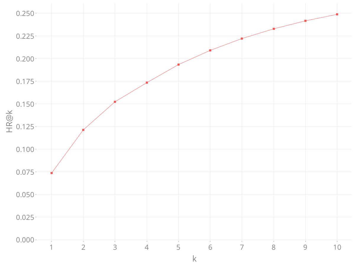
pc:mainObject4.4.4 Combined features
Having evaluated the properties individually we examined whether their combinations could perform better. We combined the properties with the baseline property pc:mainObject, using a reduced weight of 0.1 for the added properties. Besides the properties evaluated above, we also experimented with including the qualifiers of CPV concepts we described in Section 2.4.6.1. The evaluation results of the matchmakers based on the combinations of properties are presented in Table 5. None of the properties produced a significant synergistic effect with pc:mainObject. If there was an improvement, its scale was not practically meaningful. We also experimented with a larger range of weights for the combination with pc:additionalProperty, however, none of the weights led to a significant difference in the evaluation results. Our conclusion in this respect is in line with Maidel et al., who found in similar circumstances that “the inclusion of item concept weights does not improve the performance of the algorithm” (2008, p. 97).
| Property | HR@10 | MRR@10 | CC@10 | PC | LTP@10 |
|---|---|---|---|---|---|
pc:additionalObject |
0.253 | 0.124 | 0.57 | 0.99 | 0.645 |
pc:kind |
0.162 | 0.075 | 0.092 | 0.996 | 0.144 |
isvz:serviceCategory |
0.197 | 0.092 | 0.392 | 0.995 | 0.368 |
| Qualifier | 0.249 | 0.125 | 0.568 | 0.978 | 0.685 |
pc:additionalObject, qualifiers |
0.254 | 0.123 | 0.557 | 0.99 | 0.639 |
pc:additionalObject, pc:kind, isvz:serviceCategory |
0.154 | 0.072 | 0.088 | 0.996 | 0.129 |
4.4.5 Query expansion
Apart from using combinations of properties, we can also extend the baseline matchmaker via query expansion, as documented in Section 3.2.2.2. We evaluated the expansion to the related CPV concepts connected via hierarchical relations, both in the direction to broader concepts, to narrower concepts, or in both directions. The query expansion followed a given maximum number of hops in these directions. Since following too many hops to related concepts can introduce noise (Di Noia et al. 2012b), we weighted the concepts inferred by query expansion either by a fixed inhibition or by a weight derived from their IDF. The results of the experiments with query expansion are gathered in Table 6. Here, ↑ denotes the number of hops expanded to the broader concepts and ↓ indicates the hops to the narrower concepts. Expansion by one hop to broader and narrower concepts was able to improve on the accuracy metrics slightly. Overall, we found that introducing query expansion led only to minuscule changes in the performance of the baseline matchmaker. For instance, the expansion to broader concepts weighted by IDF produced results that differed only in higher decimal precision for the different numbers of hops followed.
| ↑ | ↓ | Weight | HR@10 | MRR@10 | CC@10 | PC | LTP@10 |
|---|---|---|---|---|---|---|---|
| 1 | 0 | 1 | 0.245 | 0.119 | 0.51 | 0.99 | 0.67 |
| 1 | 0 | 0.5 | 0.252 | 0.124 | 0.533 | 0.99 | 0.673 |
| 1 | 0 | 0.1 | 0.257 | 0.127 | 0.563 | 0.99 | 0.682 |
| 2 | 0 | 0.1 | 0.258 | 0.126 | 0.545 | 0.994 | 0.672 |
| 3 | 0 | 0.1 | 0.257 | 0.125 | 0.517 | 0.996 | 0.65 |
| 1 | 0 | IDF | 0.249 | 0.125 | 0.565 | 0.978 | 0.684 |
| 2 | 0 | IDF | 0.249 | 0.125 | 0.565 | 0.978 | 0.684 |
| 3 | 0 | IDF | 0.249 | 0.125 | 0.565 | 0.978 | 0.684 |
| 0 | 1 | 1 | 0.248 | 0.123 | 0.527 | 0.982 | 0.677 |
| 0 | 1 | 0.5 | 0.252 | 0.125 | 0.549 | 0.982 | 0.677 |
| 0 | 1 | 0.1 | 0.253 | 0.126 | 0.569 | 0.982 | 0.677 |
| 0 | 2 | 0.1 | 0.253 | 0.126 | 0.565 | 0.979 | 0.679 |
| 0 | 3 | 0.1 | 0.254 | 0.126 | 0.562 | 0.982 | 0.677 |
| 0 | 1 | IDF | 0.253 | 0.126 | 0.572 | 0.982 | 0.684 |
| 0 | 2 | IDF | 0.254 | 0.126 | 0.572 | 0.982 | 0.68 |
| 0 | 3 | IDF | 0.254 | 0.126 | 0.569 | 0.982 | 0.682 |
| 1 | 1 | 0.1 | 0.259 | 0.128 | 0.563 | 0.991 | 0.678 |
| 1 | 1 | IDF | 0.249 | 0.125 | 0.565 | 0.978 | 0.684 |
4.4.6 Data reduction
We evaluated the impact of data reduction on HR@10 for the baseline matchmaker and the blind matchmaker that constantly recommends the top winning bidders. Prior to running the evaluation we reduced the number of links between contracts and bidders to a given fraction. For example, if the level of data reduction was set to 0.4, 60 % of the links were removed. Links to remove were selected randomly. Fig. 14 shows the HR@10 per level of data reduction for the two compared matchmakers. In general, we decreased the data reduction level by 0.1 for each evaluation run, but a smaller step was used for the lower levels to better distinguish the impact of data reduction at smaller data sizes. The evaluation showed that HR@10 grows logarithmically with the size of the data for the baseline, while the blind matchmaker performs the same no matter the data size. As can be expected, the baseline matchmaker improves its performance as the data it learns from accrues. Both approaches suffer from the cold start problem, although the baseline matchmaker improves rapidly with the initial data growth and demonstrates diminishing returns as data becomes larger.
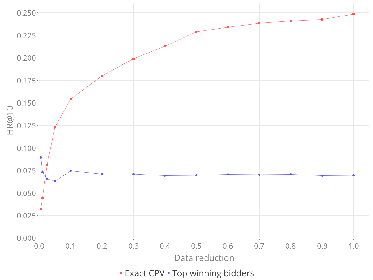
4.4.7 Data refinement
Of the data refinement steps undertaken, as described in Section 2.3, we evaluated what impact better deduplication and mapping CPV 2003 to CPV 2008 had on the baseline matchmaker. Both steps improved the evaluation results of the matchmaker, as can be seen in Table 7. Better deduplication and fusion of bidders reduces the search space of possible matches, so that the probability of finding the correct match increases. Mapping CPV 2003 to CPV 2008 enlarges the dataset the matchmaker can learn from by 15.31 %, accounting for older contracts described by CPV 2003. However, while HR@10 improves after this mapping, CC@10 decreases, which may be explained by more data affirming the few established bidders. Better deduplication improves the accuracy metrics only slightly, which may be due to the original data already being free of most duplicates. Nevertheless, in our prior work (Mynarz et al. 2015), deduplication produced the greatest improvement in the evaluation of the baseline matchmaker.
| Dataset | HR@10 | MRR@10 | CC@10 | PC | LTP@10 |
|---|---|---|---|---|---|
| Prior to CPV 2003 mapping | 0.237 | 0.12 | 0.595 | 0.931 | 0.798 |
| Prior to better deduplication | 0.245 | 0.121 | 0.554 | 0.955 | 0.858 |
| Final | 0.248 | 0.124 | 0.567 | 0.978 | 0.684 |
4.4.8 Counter-measures to limits of ground truth
We evaluated two approaches devised as counter-measures to address the limits of our ground truth we described in Section 3.1. One of them weighted contract awards by the zIndex fairness score of the contracting authority, the other limited the training dataset to the contracts awarded in open procedures. The proposed counter-measures were not successful. Both approaches fared worse than our baseline, as documented in Table 8. While the impact of weighting by zIndex is barely noticeable, the restriction to open procedures decreased most of the observed metrics. The decrease may be attributed to the smaller size of training data, even though the majority of contracts in our dataset were awarded via an open procedure.
| Matchmaker | HR@10 | MRR@10 | CC@10 | PC | LTP@10 |
|---|---|---|---|---|---|
pc:mainObject |
0.248 | 0.124 | 0.567 | 0.978 | 0.684 |
pc:mainObject, zIndex |
0.243 | 0.121 | 0.566 | 0.978 | 0.687 |
pc:mainObject, open procedures |
0.214 | 0.106 | 0.469 | 0.964 | 0.702 |
In conclusion, rather than improving on the baseline matchmaker, we managed to analyze what makes it perform well. It benefits mostly from refining and extending the training data and from using the product aggregation function. Other extensions of the baseline matchmaker were found to have little practical benefits. A slightly better results were achieved when query expansion by one hop to broader and narrower concepts was used, although this improvement was counterweighed by an increased response time. Simply put, the evaluation indicated that “simple models and a lot of data trump more elaborate models based on less data” (Halevy et al. 2009, p. 9).
4.5 Results of RESCAL-based matchmakers
The approach for exploring the space of configurations of RESCAL-based matchmakers was similar to the one used for SPARQL-based matchmakers. We started with pc:mainObject as the principal feature and examined what improvements can be achieved via adjustments of hyper-parameters, combinations with additional features, or other treatments. The adopted heuristic for tuning the matchmakers’ performance can be considered a manually guided grid search. Note that RESCAL exhibits a greater degree of non-determinism than the SPARQL-based method, so that its evaluation results have greater variance.
We measured the same evaluation metrics for the RESCAL-based matchmakers as for the SPARQL-based ones. Since we do not use any threshold for the RESCAL-based matchmakers, their prediction coverage is always maximum. Consequently, for brevity, we omit this metric from the evaluation results.
4.5.1 Hyper-parameters
The central hyper-parameter of RESCAL is the rank of its decomposition. As reported in existing research, RESCAL’s accuracy improves with increasing rank of the factorization. With higher ranks we observe diminishing returns and, eventually, HR@10 ceases to improve at around rank 500, as Fig. 15 displays. An analogous impact can be observed for CC@10, although its growth is much more subtle. We tested ranks ranging from 10 to 1000, using smaller intervals for greater resolution in low ranks. Runtime of tensor factorization with RESCAL increases approximately linearly with the rank, so there is a need to balance the quality of RESCAL’s results with the available time to compute them.
We observed that performance improves with rank only for more selective properties, e.g., pc:mainObject. Properties that have fewer distinct values, such as pc:kind, reach their peak performance already at lower ranks.
RESCAL allows to tune its generalization ability via the regularization parameters \(\lambda_{A}\) for the latent factor matrix \(A\) and \(\lambda_{R}\) for the tensor \(R\) that captures the interactions of the latent components. Increasing the amount of regularization helps avoid overfitting. Optimal values of the regularization parameters are dataset-specific. While Padia et al. (2016) achieved the best results with \(\lambda_{A} = 10\) and \(\lambda_{R} = 0.2\), Kuchař et al. (2016) obtained the peak performance by setting both to 0.01. In our case, we found that relatively high values of the regularization parameters tend to achieve the best results. We set both \(\lambda_{A}\) and \(\lambda_{R}\) to be 10. A comparison of a few selected values of the regularization parameters is shown in Table 9 for pc:mainObject at rank 50.
| \(\lambda_{A}\) | \(\lambda_{R}\) | HR@10 | MRR@10 | CC@10 | LTP@10 |
|---|---|---|---|---|---|
| 0 | 0 | 0.049 | 0.024 | 0.016 | 0.493 |
| 0.01 | 0.01 | 0.066 | 0.028 | 0.01 | 0.272 |
| 10 | 0.2 | 0.077 | 0.032 | 0.006 | 0.163 |
| 10 | 10 | 0.081 | 0.032 | 0.006 | 0.049 |
| 20 | 20 | 0.081 | 0.032 | 0.006 | 0.042 |
The remaining hyper-parameters exposed by RESCAL include initialization methods and convergence criteria. RESCAL can initialize the latent matrices either randomly or by eigenvalues of the input tensor, the latter method being clearly superior, as shown in Table 10 for pc:mainObject at rank 50. RESCAL stops when it reaches the given convergence criteria, which can be specified either as the maximum number of iterations or as the maximum residual. We used the default values for these hyper-parameters.
| Initialization method | HR@10 | MRR@10 | CC@10 | LTP@10 |
|---|---|---|---|---|
| Random | 0.002 | 0.001 | 0.003 | 1 |
| Eigenvalues | 0.081 | 0.032 | 0.006 | 0.049 |
In the further experiments, we use rank 500 and both \(\lambda_{A}\) and \(\lambda_{R}\) set to 10, unless specified otherwise.
4.5.2 Feature selection
We evaluated the predictive power of the descriptive features that can be obtained from our dataset. While most features correspond to RDF properties, some are derived from property paths, such as pc:location/schema:address or pc:awardCriteriaCombination/pc:awardCriterion/pc:weightedCriterion, which we shorten as pc:weightedCriterion. We started by assessing the results of matchmakers based on the individual features. We combined each feature with the ground truth comprising contract awards and observed how well the feature can help predict the awarded bidders. We evaluated the HR@10 of selected features at ranks 50 and 500, as shown in Fig. 16.
Out of the features pc:mainObject obtained the best results. Higher rank improves the results of most features, such as pc:mainObject, pc:contractingAuthority, or isvz:serviceCategory. However, increasing rank has the inverse effect on other features, including pc:procedureType, pc:actualPrice, or isvz:mainCriterion. We observed that features for which higher rank improves the evaluation results have higher cardinality, while the converse is usually true for features with low cardinality. Here, cardinality is the number of distinct values a feature has in a dataset. For instance, the cardinalities of the mentioned features for which results improve with the increased rank are 4588, 16982, and 43; whereas the cardinalities of the respective features that exhibit the inverse are 10, 15, and 4. These observations suggest that higher rank can reach better resolution if provided with a feature having a higher cardinality. Conversely, RESCAL cannot leverage a higher rank if given a feature with low cardinality, in which case its latent components capture noise instead of informative distinctions. Nevertheless, high cardinality does not imply good results, such as in case of pc:weightedCriterion that has 27793 distinct values in our dataset, yet achieves poor results.
| Feature | HR@10 | MRR@10 | CC@10 | LTP@10 |
|---|---|---|---|---|
ares:zivnost |
0.002 | 0 | 0.015 | 0.952 |
isvz:mainCriterion |
0.075 | 0.031 | 0.009 | 0.048 |
isvz:serviceCategory |
0.096 | 0.036 | 0.014 | 0.392 |
pc:additionalObject |
0.048 | 0.021 | 0.016 | 0.669 |
pc:contractingAuthority |
0.137 | 0.064 | 0.02 | 0.202 |
pc:kind |
0.121 | 0.051 | 0.009 | 0.003 |
pc:location/schema:address |
0.045 | 0.016 | 0.014 | 0.116 |
pc:mainObject |
0.17 | 0.077 | 0.02 | 0.211 |
pc:procedureType |
0.071 | 0.021 | 0.009 | 0.012 |
pc:weightedCriterion |
0.019 | 0.007 | 0.017 | 0.753 |
rov:orgActivity |
0.001 | 0 | 0.022 | 0.995 |
Results of all evaluation metrics for the individual features as listed in Table 11. The pc:mainObject property clearly stands out with the best results of the accuracy metrics. Although the properties of bidders, i.e. ares:zivnost and rov:orgActivity, achieve the best results for the diversity metrics, their poor accuracy is comparable to the results of random matchmaking.
As in the evaluation of the SPARQL-based matchmakers, we adopted pc:mainObject as our pivot feature that we combined with additional features. After we evaluated the features separately, our next step was to see how they perform in combination with pc:mainObject. The evaluation results of these feature pairs are shown in Table 12. In case of rdf:type we included the links to classes of public contracts and bidders. The skos:broaderTransitive property adds the hierarchical relations in CPV, thus emulating the query expansion we described in Section 3.2.2.2. The skos:related property brings in the qualifying concepts from the supplementary vocabulary of CPV.94 We achieved the best improvement in all evaluated metrics with the rov:orgActivity property that associates bidders with concepts from the NACE classification in the Business Register we covered in Section 2.4.6.2.
| Additional feature | HR@10 | MRR@10 | CC@10 | LTP@10 |
|---|---|---|---|---|
ares:zivnost |
0.171 | 0.078 | 0.023 | 0.17 |
isvz:mainCriterion |
0.152 | 0.069 | 0.022 | 0.075 |
isvz:serviceCategory |
0.172 | 0.076 | 0.021 | 0.212 |
pc:additionalObject |
0.175 | 0.079 | 0.021 | 0.177 |
pc:contractingAuthority |
0.171 | 0.083 | 0.023 | 0.215 |
pc:kind |
0.163 | 0.073 | 0.02 | 0.122 |
pc:location/schema:address |
0.172 | 0.078 | 0.02 | 0.139 |
pc:procedureType |
0.157 | 0.071 | 0.023 | 0.08 |
pc:weightedCriterion |
0.164 | 0.075 | 0.021 | 0.121 |
rdf:type |
0.154 | 0.069 | 0.013 | 0.068 |
rov:orgActivity |
0.187 | 0.083 | 0.036 | 0.295 |
skos:broaderTransitive |
0.174 | 0.079 | 0.021 | 0.156 |
skos:related |
0.173 | 0.078 | 0.02 | 0.176 |
Ultimately, we examined a larger set of features that improved the results of pc:mainObject when combined with it one by one. We tested separately a subset of the improving features that involved only the links to subject classifications via pc:mainObject, pc:additionalObject and rov:orgActivity, together with the hierarchical relations in both CPV and NACE represented by the skos:broaderTransitive property. The evaluation results for both combinations of additional features are presented in Table 13.
| Additional features | HR@10 | MRR@10 | CC@10 | LTP@10 |
|---|---|---|---|---|
pc:additionalObject, rov:orgActivity, skos:broaderTransitive |
0.182 | 0.081 | 0.044 | 0.311 |
ares:zivnost, isvz:serviceCategory, pc:additionalObject, pc:contractingAuthority, pc:location/schema:address, rov:orgActivity, skos:broaderTransitive |
0.125 | 0.065 | 0.017 | 0.208 |
The subset of subject classifications fared better than indiscriminate inclusion of all improving features. Yet still, this combination of features did not surpass the evaluation results of pc:mainObject combined just with rov:orgActivity. The worse results scored by the combinations of features individually improving the pc:mainObject baseline invalidate our assumption that the contributions of features do not cancel themselves out. To the contrary, this interplay illustrates that their contributions are not cumulative, and, in fact, some features diminish the contribution of other features.
The directionality of relations in the input tensor matters for RESCAL. We examined this characteristic using the rov:orgActivity property. In the source data, rov:orgActivity is a property of bidders associating them with NACE concepts. We found out that the evaluation results differ widely if the domain of this property changes. Apart from its directionality in the source data, we evaluated the cases in which the property is directly attached to contracts and when it is symmetric. As can be seen in Table 14, the symmetric option decidedly outperforms the others. Nevertheless, treating relations as symmetric does not always lead to an improvement, as in the case of pc:mainObject when the symmetric interpretation in fact worsens the evaluation results.
Domain of rov:orgActivity |
HR@10 | MRR@10 | CC@10 | LTP@10 |
|---|---|---|---|---|
| Bidder | 0.001 | 0 | 0.022 | 0.995 |
| Contract | 0.003 | 0.001 | 0.015 | 0.951 |
| Bidder and contract | 0.137 | 0.105 | 0.086 | 0.656 |
4.5.3 Ageing relations
Evaluation of ageing was done by time series cross-validation, as described in Section 4.2. Ageing, which we covered in Section 2.6.2, was applied to the tensor slice containing the links between public contracts and awarded bidders. We compared how ageing affects matchmaking with the pc:mainObject property. As shown in Table 15, applying the ageing worsens the results of the accuracy metrics. When compared to pc:mainObject evaluated using the n-fold cross-validation, the results in time series cross-validation are notably worse, which can be attributed to the lower volume of data available in this evaluation protocol.
| Configuration | HR@10 | MRR@10 | CC@10 | LTP@10 |
|---|---|---|---|---|
pc:mainObject |
0.07 | 0.03 | 0.013 | 0.185 |
pc:mainObject, aged |
0.035 | 0.013 | 0.016 | 0.413 |
4.5.4 Use of literals
We experimented with a limited use of literals, namely via discretization of the actual prices of contracts, represented by the pc:actualPrice property, which we split into 15 equifrequent intervals having approximately the same number of members. Actual prices were known for 91.5 % of contracts in the evaluated dataset. We combined the discretized actual prices with pc:mainObject. A comparison of the combination with pc:mainObject only is shown in Table 16. Adding actual prices mostly worsens the evaluation results. We surmise that the decrease can be explained by noisy data about prices. Upon manual inspection, we found that prices may be reported as coefficients to be multiplied by an implicit factor that is not part of the structured data.
| Features | HR@10 | MRR@10 | CC@10 | LTP@10 |
|---|---|---|---|---|
pc:actualPrice |
0.078 | 0.028 | 0.013 | 0.083 |
pc:mainObject |
0.17 | 0.077 | 0.02 | 0.211 |
pc:mainObject, pc:actualPrice |
0.155 | 0.07 | 0.025 | 0.086 |
In summary, the best results in RESCAL-based matchmakers were achieved for pc:mainObject combined with rov:orgActivity. These relations linking subject classifications, i.e. CPV and NACE, turned out to be the most informative for the prediction of awarded bidders. We found that rank 500 tends to deliver the best accuracy, especially if combined with relatively high regularization parameters that prevent overfitting.
4.6 Comparison of the results
When we compared the evaluation results of the SPARQL-based and the RESCAL-based matchmakers, we could see that both approaches were largely in line with each other. Both highlighted pc:mainObject as the principal feature for matchmaking. Both found the highest predictive power in subject classifications with controlled vocabularies. Overall, the RESCAL-based matchmakers produced results with very low diversity, especially when considering their CC@10. The low diversity means that they tend to recommend the same bidders repeatedly, the shortcoming we did not observe in most of the SPARQL-based matchmakers. The gap between the evaluated approaches to matchmaking was not as pronounced in accuracy metrics, although for them the RESCAL-based matchmakers also delivered inferior results.
The best SPARQL-based matchmaker used pc:mainObject with query expansion by 1 hop to both broader and narrower CPV concepts that were associated with the weight of 0.1. The best RESCAL-based matchmaker employed pc:mainObject in combination with rov:orgActivity. Both best-performing matchmakers merged features from multiple linked datasets. The SPARQL-based one added the CPV hierarchy to the Czech public procurement dataset, while the RESCAL-based one combined the procurement data with the Business Register.
| Matchmaker | HR@10 | MRR@10 | CC@10 | PC | LTP@10 |
|---|---|---|---|---|---|
| SPARQL | 0.259 | 0.128 | 0.563 | 0.991 | 0.678 |
| RESCAL | 0.187 | 0.083 | 0.036 | 1 | 0.295 |
As shown in Table 17, the best SPARQL-based matchmaker clearly outmatches the best RESCAL-based matchmaker both in terms of accuracy and diversity. Moreover, the SPARQL-based matchmaker also excels in performance and the ability to handle real-time queries.
5 Conclusions
In conclusion, we summarize our work and review it in hindsight from several perspectives. We sum up our main contributions and contrast them with the current research to indicate our progress beyond the state of the art. We consider the practical applicability of our work and provide concrete examples of incorporating it into end-user applications. Finally, we assess the degree of fulfilment of our stated goals and suggest directions for future research.
5.1 Main contributions
We developed and documented methods to match public contracts to bidders. These methods leverage linked open data that describes the entities involved in matchmaking as being a part of a semantically described knowledge graph, which includes descriptions of the entities, as well as their interactions, relations, or contextual data. We implemented the proposed matchmaking methods by using existing technologies, namely SPARQL, an RDF query language, and RESCAL, a tensor factorization algorithm. The implementations served as artefacts that we experimented with. We examined their usefulness by evaluating the accuracy and diversity of the matches they produce.
In order to approximate the conditions in real-world public procurement we evaluated the designed matchmaking methods on a large dataset of retrospective data spanning ten years of Czech public procurement, including several related datasets. Preparation of this dataset constituted a fundamental part of our work. Transforming the data into a knowledge base structured as linked open data required an extensive effort that warranted the development of novel and reusable tools for data processing. Both the prepared dataset and the developed tools thus represent a key side contribution of our research. We published the cleaned and enriched Czech public procurement dataset as linked open data for anyone to reuse. Similarly, the implemented tools for working with RDF data were released as open source.
The evaluation proved it challenging to obtain good results for the matchmaking task. Already during data preparation, we discovered the underlying data to be riddled with errors and ambiguity. Moreover, we problematized the ground truth that the matchmakers use to learn about matching public contracts to bidders. As we explained, the ground truth comprising data on historical awards of public contracts is subject to systemic biases that undermine its relevance for matchmaking. Despite these shortcomings, the evaluation indicated that the SPARQL-based matchmakers can be used to pre-screen relevant bidders or public contracts. Moreover, they can answer matchmaking queries on demand, even on constantly updating data. Apart from having subpar accuracy, the results of the RESCAL-based matchmakers were afflicted with very low diversity. These matchmakers turned out to be inferior in all the evaluated respects when compared with the SPARQL-based ones. We found the assumption that contextual data can improve matchmaking to be justified, although the improvements proceeding from incorporating additional linked data turned out to be relatively minor. Nevertheless, most linked open data must be considered to be raw data that requires significant data preparation effort to realize its effective use.
5.2 Progress beyond the state of the art
When we review our progress beyond the state of the art, introduced in Section 1.7, our key contribution is the adaptation of existing generic technologies for a concrete use case concerning matchmaking in the Czech public procurement. Using SPARQL, we developed a novel matchmaking method inspired by case-based reasoning. The closest to this method is the work of Alvarez-Rodríguez et al. (2011b), which is however documented only in broad strokes, thus preventing more detailed comparison. The combination of logical deduction and statistical learning we were inspired by can be traced back to the work on iSPARQL by Kiefer and Bernstein (2008). The RESCAL-based matchmakers build on the generic basis laid out by the Web of Needs (Friedrich 2015), combining it with novel extensions and specialization to the public procurement domain. As a side effect of our investigation in matchmaking methods, we advanced the available means of processing RDF data by developing a set of reusable tools that address some of the recurrent tasks involved in handling RDF data. Ultimately, our work produced a greater value in the developed reusable artefacts for data preparation and matchmaking than as a practical use case in public procurement.
The presented work was built on open source software as well as data prepared by others. In particular, most of the transformations of the ARES dataset were done by Jakub Klímek. The extracted Business Register data was provided by Ondřej Kokeš. Both these contributions are acknowledged directly in Section 2.4.6.2. zIndex fairness scores were supplied to us by Datlab s.r.o. The software we reused in our work is listed in Appendix 6. The design of the Public Contracts Ontology was a collaborative effort as indicated in the references in Section 2.1.1.
5.3 Applicability of the work
The practical applicability of our work stems from the software we developed. We made both the matchmakers and the data processing tools available as open source software. The software is thus open to reuse and adaptation. In this way, we contributed back to the open source ecosystem from which we drawn tools to build on. However, while the data processing tools were designed to be reusable, the matchmakers are tied with our evaluation protocol, so they would need to be reworked for reuse. If adapted, matchmakers can be integrated with practical applications for managing public contracts, such as with our prototype described in Mynarz et al. (2014), or with zInfo.cz, a Czech platform for public contracts maintained by Datlab s.r.o.
5.4 Fulfilment of the stated goals
As stated in our goals, we explored the ways of matching of public contracts to bidders when their interactions are described as linked open data. Since the space of possibilities of applying matchmaking in this setting is vast, we managed to explore only a fraction of this space. In that light, our work can seem incomplete because the exploration has no clear boundaries. In order to maximize the information gathered in the exploration, we used heuristics to navigate the space of possibilities and select the more salient and informative features to explore.
5.5 Future work
Overall, we explored only a handful of ways of matching public contracts to bidders. Our work suggests that investing in improving the data quality may produce the highest returns. Adaptation of different approaches for the matchmaking tasks may also fundamentally alter the characteristics of matchmakers. In particular, we expect methods that are better able to leverage unstructured data in literals to determine the similarity of public contracts, such as full-text search in semi-structured data, to have a considerable potential to improve the results of matchmaking. Alternatively, matchmakers can build on other promising approaches for statistical relational learning from linked data, such as Bordes et al. (2013). Ultimately, many more ways of relevance engineering for the task of matchmaking are left open to pursue and assess their worth. However, assessing matchmakers on the task of prediction of the awarded bidders may turn out to be a false compass. As we discussed at length in Section 3.1, this evaluation setup using retrospective data on contract awards is subject to many shortcomings. Alternative ways of evaluation may bypass the weaknesses of this setup, possibly by conducting an online evaluation with real users or by involving domain experts in qualitative evaluation. Thorough examination of these alternatives for evaluation is imperative for further investigation of matchmaking methods.
References
ABELE, Andrejs, John P. MCCRAE, Paul BUITELAAR, Anja JENTZSCH and Richard CYGANIAK, 2017. Linking open data cloud diagram [online] [accessed 2017-03-02]. Available at: http://lod-cloud.net
ACCESS INFO EUROPE and OPEN KNOWLEDGE FOUNDATION, 2011. Beyond access: Open government data & the right to (re)use public information [online] [accessed 2017-01-03]. Available at: http://www.access-info.org/documents/Access_Docs/Advancing/Beyond_Access_7_January_2011_web.pdf
ADOMAVICIUS, Gediminas and YoungOk KWON, 2012. Improving aggregate recommendation diversity using ranking-based techniques. IEEE Transactions on Knowledge and Data Engineering. May 2012, 24(5), 896–911.
AKOKA, Jacky, Laure BERTI-ÉQUILLE, Omar BOUCELMA, Mokrane BOUZEGHOUB, Isabelle COMYN-WATTIAU, Mireille COSQUER, Virginie GOASDOUÉ-THION, Zoubida KEDAD, Sylvaine NUGIER, Verónika PERALTA and Samira SISAID-CHERFI, 2007. A framework for data quality evaluation in data integration systems. In: 9th international conference on enterprise information systems [online]. p. 170–175. Available at: http://l1.lamsade.dauphine.fr/scripts/FILES/publi1091.pdf
ALVAREZ-RODRÍGUEZ, Jose María, José Emilio LABRA GAYO and Patricia ORDOÑEZ DE PABLOS, 2013. Enabling the matchmaking of organizations and public procurement notices by means of linked open data. In: Patricia ORDOÑEZ DE PABLOS, Miltiadis LYTRAS D., Robert TENNYSON D. and José Emilio LABRA GAYO, eds. Cases on open-linked data and semantic web applications [online]. Hershey (PA): IGI Global, p. 105–131. Available at: doi:10.4018/978-1-4666-2827-4.ch006
ALVAREZ-RODRÍGUEZ, Jose María, José Emilio LABRA GAYO, Ramón CALMEAU, Ángel MARÍN and Jose Luis MARÍN, 2011a. Innovative services to ease the access to the public procurement notices using linking open data and advanced methods based on semantics. In: Proceedings of the 5th international conference on methodologies and tools enabling e-government [online]. Available at: http://www.josemalvarez.es/web/mypapers/metteg2011.pdf
ALVAREZ-RODRÍGUEZ, Jose María, José Emilio LABRA GAYO, Ramón CALMEAU, Ángel MARÍN and Jose Luis MARÍN, 2011b. Query expansion methods and performance: Evaluation for reusing linking open data of the european public procurement notices. In: Jose A. LOZANO, José A. GÁMEZ and José A. MORENO, eds. Advances in artificial intelligence: Proceedings of the 14th conference of the spanish association for artificial intelligence [online]. Berlin; Heidelberg: Springer. Lecture notes in computer science. ISBN 978-3-642-25273-0. Available at: doi:10.1007/978-3-642-25274-7
ALVAREZ-RODRÍGUEZ, Jose María, José Emilio LABRA GAYO, Francisco CIFUENTES, Gilor ALOR-HÉRNANDEZ, Cuauhtémoc SÁNCHEZ and Jaime Alberto GUZMÁN LUNA, 2012. Towards a pan-european e-procurement platform to aggregate, publish and search public procurement notices powered by linked open data: The MOLDEAS approach. International Journal of Software Engineering and Knowledge Engineering [online]. 2012, 22(3). Available at: doi:10.1142/S0218194012400086
ALVAREZ-RODRÍGUEZ, Jose María, José Emilio LABRA GAYO, Ángel MARÍN and Jose Luis MARÍN, 2011c. Semantic methods for reusing linking open data of the european public procurement notices. In: Extended semantic web conference 2011 PhD symposium [online]. Available at: http://www.josemalvarez.es/mypapers/eswc2011phdsymposium.pdf
ALVAREZ-RODRÍGUEZ, Jose María, José Emilio LABRA-GAYO and Patricia ORDOÑEZ DE PABLOS, 2014. New trends on e-procurement applying semantic technologies: Current status and future challenges. Computers in Industry [online]. 2014, 65(5), 800–820. Available at: doi:10.1016/j.compind.2014.04.005
ANKOLEKAR, Anupriya, Mark BURSTEIN, Jerry R. HOBBS, Ora LASSILA, David MARTIN, Drew MCDERMOTT, Sheila A. MCILRAITH, Srini NARAYANAN, Massimo PAOLUCCI, Terry PAYNE and Katia SYCARA, 2002. DAML-S: Web service description for the semantic web. In: Ian HORROCKS and James HENDLER, eds. The semantic web: Proceedings of the first international semantic web conference [online]. Berlin; Heidelberg: Springer, p. 348–363. Lecture notes in computer science. ISBN 978-3-540-43760-4. Available at: doi:10.1007/3-540-48005-6_27
ARCHER, Phil, Marios MEIMARIS and Agisilaos PAPANTONIOU, eds., 2013. Registered organization vocabulary [online]. W3C Working Group Note. [accessed 2017-01-01]. Available at: https://www.w3.org/TR/vocab-regorg
AYERS, Danny, 2007. Evolving the link. IEEE Internet Computing. 2007, 11(1), 94–96. ISSN 1089-7801.
BANDIERA, Oriana, Andrea PRAT and Tommaso VALLETTI, 2009. Active and passive waste in government spending: Evidence from a policy experiment. American Economic Review [online]. 2009, 99(4), 1278–1308. Available at: doi:10.1257/aer.99.4.1278
BATINI, Carlo and Monica SCANNAPIECO, 2006. Data quality: Concepts, methodologies and techniques. Berlin; Heidelberg: Springer. Data-centric systems and applications. ISBN 978-3-540-33173-5.
BECKETT, David, Tim BERNERS-LEE, Eric PRUD’HOMMEAUX and Gavin CAROTHERS, 2014. RDF 1.1 Turtle: Terse RDF triple language [online]. W3C Recommendation. [accessed 2017-02-17]. Available at: https://www.w3.org/TR/turtle
BEEL, Joeran, Stefan LANGER, Bela GIPP, Marcel GENZMEHR and Andreas NÜRNBERGER, 2013. A comparative analysis of offline and online evaluations and discussion of research paper recommender system evaluation. In: Proceedings of the international workshop on reproducibility and replication in recommender systems evaluation [online]. New York (NY): ACM, p. 7–14. ISBN 978-1-4503-2465-6. Available at: doi:10.1145/2532508.2532511
BELIAKOV, Gleb, Tommaso CALVO and Simon JAMES, 2015. Aggregation functions for recommender systems. In: Francesco RICCI, Lior ROKACH and Bracha SHAPIRA, eds. Recommender systems handbook [online]. 2nd ed. Berlin; Heidelberg: Springer, p. 777–808. Available at: doi:10.1007/978-1-4899-7637-6_23
BERNERS-LEE, Tim, 1996. Universal resource identifiers: Axioms of web architecture [online] [accessed 2017-01-01]. Available at: http://www.w3.org/DesignIssues/Axioms.html
BERNERS-LEE, Tim, 2009. Linked data: Design issues [online] [accessed 2017-02-16]. Available at: http://www.w3.org/DesignIssues/LinkedData.html
BIZER, Christian, Tom HEATH and Tim BERNERS-LEE, 2009. Linked data: The story so far. International Journal on Semantic Web and Information Systems [online]. 2009, 5(3), 1–22. Available at: doi:10.4018/jswis.2009081901
BLEIHOLDER, Jens and Felix NAUMANN, 2006. Conflict handling strategies in an integrated information system. In: Proceedings of the WWW 2006 workshop in information integration on the web (IIWEB) [online]. Available at: http://edoc.hu-berlin.de/series/informatik-berichte/197/PDF/197.pdf
BLEIHOLDER, Jens and Felix NAUMANN, 2008. Data fusion. ACM Computing Surveys [online]. 2008, 41(1). Available at: doi:10.1145/1456650.1456651
BONCZ, Peter, Orri ERLING and Minh-Duc PHAM, 2014. Advances in large-scale RDF data management. In: Sören AUER, Volha BRYL and Sebastian TRAMP, eds. Linked open data: Creating knowledge out of interlinked data [online]. Berlin; Heidelberg: Springer, Lecture notes in computer science, p. 21–44. ISBN 978-3-319-09845-6. Available at: doi:10.1007/978-3-319-09846-3_2
BORDES, Antoine, Nicolas USUNIER, Alberto GARCIA-DURAN, Jason WESTON and Oksana YAKHNENKO, 2013. Translating embeddings for modeling multi-relational data. In: C. J. C. BURGES, L. BOTTOU, M. WELLING, Z. GHAHRAMANI and K. Q. WEINBERGER, eds. Advances in neural information processing systems [online]. Curran Associates, p. 2787–2795. Available at: http://papers.nips.cc/paper/5071-translating-embeddings-for-modeling-multi-relational-data.pdf
BRICKLEY, Dan, 2002. RDF: Understanding the striped RDF/XML syntax [online] [accessed 2017-01-13]. Available at: https://www.w3.org/2001/10/stripes
BRICKLEY, Dan and Ramanathan V. GUHA, eds., 2014. RDF Schema 1.1 [online]. W3C Recommendation. [accessed 2017-02-17]. Available at: https://www.w3.org/TR/rdf-schema
BRYL, Volha, Christian BIZER, Robert ISELE, Mateja VERLIC, Soon Gill HONG, Sammy JANG, Mun Yong YI and Key-Sun CHOI, 2014. Interlinking and knowledge fusion. In: Sören AUER, Volha BRYL and Sebastian TRAMP, eds. Linked open data: Creating knowledge out of interlinked data [online]. Berlin; Heidelberg: Springer, Lecture notes in computer science, p. 70–89. ISBN 978-3-319-09845-6. Available at: doi:10.1007/978-3-319-09846-3_2
CAROTHERS, Gavin, ed., 2014. RDF 1.1 N-Quads: A line-based syntax for RDF datasets [online]. W3C Recommendation. [accessed 2017-02-17]. Available at: https://www.w3.org/TR/n-quads
CHANG, Kai-Wei, Scott Wen-tau YIH, Bishan YANG and Chris MEEK, 2014. Typed tensor decomposition of knowledge bases for relation extraction. In: Proceedings of the 2014 conference on empirical methods in natural language processing [online]. ACL – Association for Computational Linguistics. Available at: https://www.microsoft.com/en-us/research/publication/typed-tensor-decomposition-of-knowledge-bases-for-relation-extraction
CHRISTEN, Peter, 2012. Data matching: Concepts and techniques for record linkage, entity resolution, and duplicate detection [online]. Berlin; Heidelberg: Springer. Data-centric systems and applications. Available at: doi:10.1007/978-3-642-31164-2
CRASWELL, Nick, 2009. Mean reciprocal rank. In: Ling LIU and Tamer ÖZSU, eds. Encyclopedia of database systems. Berlin; Heidelberg: Springer, p. 1703. ISBN 978-0-387-39940-9.
CYGANIAK, Richard and Dave REYNOLDS, eds., 2014. The RDF Data Cube Vocabulary [online]. W3C Recommendation. [accessed 2017-01-24]. Available at: https://www.w3.org/TR/vocab-data-cube
CYGANIAK, Richard, David WOOD and Markus LANTHALER, eds., 2014. RDF 1.1 concepts and abstract syntax [online]. W3C Recommendation. [accessed 2017-02-17]. Available at: http://www.w3.org/TR/rdf11-concepts
CZECH REPUBLIC, 2016. Zákon č. 134/2016 sb., zákon o zadávání veřejných zakázek. 2016. ISSN 0322‑8037.
DAVIES, John, Alistair DUKE and Atanas KIRIYAKOV, 2009. Semantic search. In: Ayse GÖKER and John DAVIES, eds. Information retrieval: Searching in the 21st century. Chichester (UK): John Wiley & Sons, p. 179–213. ISBN 978-0-470-03364-7.
DELBRU, Renaud, Stephane CAMPINAS and Giovanni TUMMARELLO, 2012. Searching web data: An entity retrieval and high-performance indexing model. Web Semantics [online]. 2012, 10, 33–58. ISSN 1570-8268. Available at: doi:10.1016/j.websem.2011.04.004
DESHPANDE, Mukund and George KARYPIS, 2004. Item-based top-n recommendation algorithms. ACM Transactions on Information Systems [online]. January 2004, 22(1), 143–177. ISSN 1046-8188. Available at: doi:10.1145/963770.963776
DI NOIA, Tommaso and Vito Claudio OSTUNI, 2015. Recommender systems and linked open data. In: Wolfgang FABER and Adrian PASCHKE, eds. Reasoning web. web logic rules. 11th international summer school 2015 [online]. Berlin; Heidelberg: Springer, p. 88–113. Lecture notes in computer science. Available at: http://sisinflab.poliba.it/publications/2015/DO15/Recommender%20Systems%20and%20Linked%20Open%20Data%20-%20RW%202015.pdf
DI NOIA, Tommaso, Ivan CANTADOR and Vito Claudio OSTUNI, 2014. Linked open data-enabled recommender systems: ESWC 2014 challenge on book recommendation. In: Valentina PRESUTTI, Milan STANKOVIC, Eric CAMBRIA, Iván CANTADOR, Angelo DI IORIO, Tommaso DI NOIA, Christoph LANGE, Diego REFORGIATO RECUPERO and Anna TORDAI, eds. Semantic web evaluation challenge: Revised selected papers. Berlin; Heidelberg: Springer, p. 129–143. Communications in computer and information science.
DI NOIA, Tommaso, Eugenio DI SCIASCIO and Francesco M. DONINI, 2007. Semantic matchmaking as non-monotonic reasoning: A description logic approach. Journal of Artificial Intelligence Research [online]. May 2007, 29(1), 269–307. ISSN 1076-9757. Available at: https://vvvvw.aaai.org/Papers/JAIR/Vol29/JAIR-2909.pdf
DI NOIA, Tommaso, Roberto MIRIZZI, Vito Claudio OSTUNI and Davide ROMITO, 2012a. Exploiting the web of data in model-based recommender systems. In: Proceedings of the 6th ACM conference on recommender systems [online]. New York (NY): ACM, p. 253–256. ISBN 978-1-4503-1270-7. Available at: doi:10.1145/2365952.2366007
DI NOIA, Tommaso, Roberto MIRIZZI, Vito Claudio OSTUNI, Davide ROMITO and Markus ZANKER, 2012b. Linked open data to support content-based recommender systems. In: Proceedings of the 8th international conference on semantic systems [online]. New York (NY): ACM, p. 1–8. ISBN 978-1-4503-1112-0. Available at: doi:10.1145/2362499.2362501
DI NOIA, Tommaso, Vito Claudio OSTUNI, Paolo TOMEO and Eugenio DI SCIASCIO, 2016. SPrank: Semantic path-based ranking for top-n recommendations using linked open data. ACM Transactions on Intelligent Systems and Technology. 2016, 8(1). ISSN 2157-6904.
DI NOIA, Tommasso, Eugenio DI SCIASCIO, Francesco M. DONINI and Marina MONGIELLO, 2004. A system for principled matchmaking in an electronic marketplace. International Journal of Electronic Commerce. 2004, 8(4), 9–37. ISSN 1557-9301.
DISTINTO, Isabella, Mathieu D’AQUIN and Enrico MOTTA, 2016. LOTED2: An ontology of european public procurement notices. Semantic Web Journal [online]. 2016, 7(3). Available at: http://oro.open.ac.uk/45732/1/swj678_0.pdf
ERLING, Orri, 2012. Virtuoso, a hybrid RDBMS/graph column store. Bulletin of the IEEE Computer Society Technical Committee on Data Engineering [online]. IEEE, March 2012, 35(1) [accessed 2017-03-04]. Available at: http://sites.computer.org/debull/A12mar/p3.pdf
EU, 2004. Directive 2004/18/EC of the European Parliament and of the Council of 31 March 2004 on the coordination of procedures for the award of public works contracts, public supply contracts and public service contracts [online]. 2004. Available at: http://data.europa.eu/eli/dir/2004/18/oj
EU, 2013. Directive 2013/37/EU of the European Parliament and of the Council of 26 June 2013 amending the Directive 2003/98/EU on the re-use of public sector information [online]. 2013. ISSN 1725-2555. Available at: http://data.europa.eu/eli/dir/2013/37/oj
EU, 2014a. Directive 2014/24/EU of the European Parliament and of the Council of 26 February 2014 on public procurement and repealing Directive 2004/18/EC [online]. 2014. Available at: http://data.europa.eu/eli/dir/2014/24/oj
EU, 2014b. Directive 2014/25/EU of the European Parliament and of the Council of 26 February 2014 on procurement by entities operating in the water, energy, transport and postal services sectors and repealing Directive 2004/17/EC [online]. 2014. Available at: http://data.europa.eu/eli/dir/2014/25/oj
EUROPEAN COMMISSION, 2016. Public procurement indicators 2015 [online] [accessed 2017-01-09]. Available at: http://ec.europa.eu/DocsRoom/documents/20679/attachments/1/translations/en/renditions/native
EUZENAT, Jérôme and Pavel SHVAIKO, 2013. Ontology matching. 2nd ed. Berlin; Heidelberg: Springer. ISBN 978-3-642-38720-3.
FEIGENBAUM, Lee, Gregory Todd WILLIAMS, Kendall Grant CLARK and Elias TORRES, eds., 2013. SPARQL 1.1 protocol [online]. W3C Recommendation. [accessed 2017-01-16]. Available at: https://www.w3.org/TR/sparql11-protocol
FRANZ, Thomas, Antje SCHULTZ, Sergej SIZOV and Steffen STAAB, 2009. TripleRank: Ranking semantic web data by tensor decomposition. In: Abraham BERNSTEIN, David R. KARGER, Tom HEATH, Lee FEIGENBAUM, Diana MAYNARD, Enrico MOTTA and Krishnaprasad THIRUNARAYAN, eds. The semantic web - ISWC 2009: 8th international semantic web conference, ISWC 2009: Proceedings [online]. Berlin; Heidelberg: Springer, p. 213–228. ISBN 978-3-642-04930-9. Available at: doi:10.1007/978-3-642-04930-9_14
FRIEDRICH, Heiko, 2015. Evaluation of tensor-based machine learning algorithms for matching human need descriptions [online]. c01. Research Studios Austria [accessed 2017-03-06]. Available at: https://sat.researchstudio.at/sites/sat.researchstudio.at/files/matching_technical_report_c012015_2.4_hf_150922.pdf
FRIEDRICH, Heiko, Florian KLEEDORFER, Soheil HUMAN and Christian HUEMER, 2016. Integrating matching services into the Web of Needs. In: Michael MARTIN, Martí CUQUET and Erwin FOLMER, eds. Joint proceedings of the posters and demos track of the 12th international conference on semantic systems - SEMANTiCS2016 and the 1st international workshop on semantic change & evolving semantics (SuCCESS’16) co-located with the 12th international conference on semantic systems (SEMANTiCS 2016) [online]. Aachen: RWTH Aachen University. CEUR workshop proceedings. Available at: http://ceur-ws.org/Vol-1695/paper19.pdf
FUTIA, Giuseppe, Alessio MELANDRI, Antonio VETRÒ, Federico MORANDO and Juan Carlos DE MARTIN, 2017. Removing barriers to transparency: A case study on the use of semantic technologies to tackle procurement data inconsistency. In: Eva BLOMQVIST, Diana MAYNARD, Aldo GANGEMI, Rinke HOEKSTRA, Pascal HITZLER and Olaf HARTIG, eds. The semantic web: 14th international conference: Proceedings, part i [online]. Cham: Springer, p. 623–637. ISBN 978-3-319-58068-5. Available at: doi:10.1007/978-3-319-58068-5_38
GANDON, Fabien and Guus SCHREIBER, eds., 2014. RDF 1.1 XML syntax [online]. W3C Recommendation. [accessed 2017-01-13]. Available at: https://www.w3.org/TR/rdf-syntax-grammar
GARCIN, Florent, Boi FALTINGS, Olivier DONATSCH, Ayar ALAZZAWI, Christophe BRUTTIN and Amr HUBER, 2014. Offline and online evaluation of news recommender systems at swissinfo.ch. In: Proceedings of the 8th ACM conference on recommender systems [online]. New York (NY): ACM, p. 169–176. ISBN 978-1-4503-2668-1. Available at: doi:10.1145/2645710.2645745
GE, Mouzhi, Carla DELGADO-BATTENFELD and Dietmar JANNACH, 2010. Beyond accuracy: Evaluating recommender systems by coverage and serendipity. In: Proceedings of the 4th ACM conference on recommender systems [online]. New York (NY): ACM, p. 257–260. ISBN 978-1-60558-906-0. Available at: doi:10.1145/1864708.1864761
GEARON, Paula, Alexandre PASSANT and Axel POLLERES, eds., 2013. SPARQL 1.1 update [online]. W3C Recommendation. [accessed 2017-02-21]. Available at: https://www.w3.org/TR/sparql11-update
GOLDBERG, Daniel W., Morven BALLARD, James H. BOYD, Narelle MULLAN, Carol GARFIELD, Diana ROSMAN and Anna M. FERRANTE, 2013. An evaluation framework for comparing geocoding systems. International Journal of Health Geographics [online]. 2013 [accessed 2017-01-05]. Available at: doi:10.1186/1476-072X-12-50
GONZÁLEZ-CASTILLO, Javier, David TRASTOUR and Claudio BARTOLINI, 2001. Description logics for matchmaking of services [online]. Hewlett-Packard [accessed 2017-03-03]. Available at: https://www.hpl.external.hp.com/techreports/2001/HPL-2001-265.pdf
GOSAIN, Sanjay, 2003. Realizing the vision for web services: Strategies for dealing with imperfect standards. In: John L. KING and Kalle LYYTINEN, eds. Proceedings of the workshop on standard making: A critical research frontier for information systems [online]. p. 10–29. Available at: http://www.joelwest.org/misq-stds/proceedings/126_10-29.pdf
GRAUX, Hans and Kronenburg TOM, 2012. State of play: Re-use of public procurement data [online]. European Public Sector Information Platform Topic Report 2012/7. [accessed 2017-02-10]. Available at: https://www.europeandataportal.eu/sites/default/files/2012_re_use_of_public_procurement_data.pdf
GRUBER, Thomas R., 1993. A translation approach to portable ontology specifications. Knowledge Acquisition [online]. 1993, 5(2), 199–220. Available at: http://tomgruber.org/writing/ontolingua-kaj-1993.htm
HAARSLEV, Volker and Ralf MÖLLER, 2001. RACER system description. In: Automated reasoning: Proceedings of the first international joint conference, IJCAR [online]. Berlin; Heidelberg: Springer, p. 701–705. Lecture notes in computer science. ISBN 978-3-540-42254-9. Available at: doi:10.1007/3-540-45744-5_59
HALEVY, Alon, Peter NORVIG and Fernando PEREIRA, 2009. The unreasonable effectiveness of data. IEEE Intelligent Systems [online]. IEEE, 2009, 24(2), 8–12. ISSN 1541-1672. Available at: doi:10.1109/MIS.2009.36
HARRIS, Steve and Andy SEABORNE, 2013. SPARQL 1.1 query language [online]. W3C Recommendation. [accessed 2017-01-03]. Available at: http://www.w3.org/TR/sparql11-query
HEATH, Tom and Christian BIZER, 2011. Linked data: Evolving the web into a global data space [online]. 1st ed. Morgan & Claypool. Synthesis lectures on the semantic web: Theory and technology. ISBN 978-1-60845-431-0. Available at: doi:10.2200/S00334ED1V01Y201102WBE001
HEBELER, John, Matthew FISHER, Ryan BLACE and Andrew PEREZ-LOPEZ, 2009. Semantic web programming. Hoboken (NJ): John Wiley & Sons. ISBN 978-0-470-41801-7.
HEITMANN, Benjamin and Connor HAYES, 2010. Using linked data to build open, collaborative recommender systems. In: Proceedings of the 2010 AAAI spring symposium: Linked data meets artificial intelligence [online]. Palo Alto (CA): AAAI, p. 76–81. Available at: http://www.aaai.org/ocs/index.php/SSS/SSS10/paper/view/1067/1452
HEITMANN, Benjamin and Conor HAYES, 2014. SemStim at the LOD-RecSys 2014 challenge. In: Valentina PRESUTTI, Milan STANKOVIC, Eric CAMBRIA, Iván CANTADOR, Angelo DI IORIO, Tommaso DI NOIA, Christoph LANGE, Diego REFORGIATO RECUPERO and Anna TORDAI, eds. Semantic web evaluation challenge: Revised selected papers [online]. Berlin; Heidelberg: Springer, p. 170–175. Communications in computer and information science. Available at: doi:10.1007/978-3-319-12024-9_22
HEITMANN, Benjamin and Conor HAYES, 2016. SemStim: Exploiting knowledge graphs for cross-domain recommendation. In: 2016 IEEE 16th international conference on data mining workshops [online]. New York (NY): IEEE, p. 999–1006. Available at: doi:10.1109/ICDMW.2016.0145
HEPP, Martin, 2008. GoodRelations: An ontology for describing products and services offers on the web. In: Knowledge engineering: Practice and patterns: Proceedings of the 16th international conference, ekaw 2008 [online]. Berlin; Heidelberg: Springer, p. 329–346. Available at: doi:10.1007/978-3-540-87696-0_29
HERLOCKER, Jonathan L., Joseph A. KONSTAN, Loren G. TERVEEN and John T. RIEDL, 2004. Evaluating collaborative filtering recommender systems. ACM Transactions on Information Systems [online]. New York (NY): ACM, January 2004, 22(1), 5–53. Available at: doi:10.1145/963770.963772
HEVNER, Alan R., Salvatore T. MARCH and Jinsoo PARK, 2004. Design science in information systems research. MIS Quarterly. January 2004, 28(1), 75–105.
HITZLER, Pascal and Frank VAN HARMELEN, 2010. A reasonable semantic web. Semantic Web [online]. 2010, 1(1, 2), 39–44. Available at: doi:10.3233/SW-2010-0010
ISELE, Robert and Christian BIZER, 2013. Active learning of expressive linkage rules using genetic programming. Web Semantics [online]. December 2013, 23, 2–15. Available at: http://www.websemanticsjournal.org/index.php/ps/article/viewFile/340/360
ISELE, Robert, Anja JENTZSCH and Christian BIZER, 2011. Efficient multidimensional blocking for link discovery without losing recall. In: Amélie MARIAN and Vasilis VASSALOS, eds. Proceedings of the 14th international workshop on the web and databases [online]. Available at: http://www.wiwiss.fu-berlin.de/en/fachbereich/bwl/pwo/bizer/research/publications/IseleJentzschBizer-WebDB2011.pdf
JACOBS, Ian and Norman WALSH, 2004. Architecture of the World Wide Web, volume 1 [online]. W3C Recommendation. [accessed 2017-01-19]. Available at: http://www.w3.org/TR/webarch
JANNACH, Dietmar, Markus ZANKER, Alexander FELFERNIG and Gerhard FRIEDRICH, 2010. Recommender systems: An introduction. 1st ed. New York (NY): Cambridge University Press. ISBN 978-0-521-49336-9.
KENNY, Charles and Jonathan KARVER, 2012. CDG policy paper: Publish what you buy: The case for routine publication of government contracts [online]. 011. Washington DC: Center for Global Development [accessed 2017-01-03]. Available at: http://www.cgdev.org/content/publications/detail/1426431
KIEFER, Christoph and Abraham BERNSTEIN, 2008. The creation and evaluation of iSPARQL strategies for matchmaking. In: The semantic web: Research and applications: Proceedings of the 5th european semantic web conference, ESWC 2008 [online]. Berlin; Heidelberg: Springer, p. 463–477. Lecture notes in computer science. ISBN 978-3-540-68233-2. Available at: doi:10.1007/978-3-540-68234-9_35
KIEFER, Christoph, Abraham BERNSTEIN and Markus STOCKER, 2007. The fundamentals of iSPARQL: A virtual triple approach for similarity-based semantic web tasks. In: Karl ABERER, Key-Sun CHOI, Natasha NOY, Dean ALLEMANG, Kyung-Il LEE, Lyndon NIXON, Jennifer GOLBECK, Peter MIKA, Diana MAYNARD, Riichiro MIZOGUCHI, Guus SCHREIBER and Philippe CUDRÉ-MAUROUX, eds. The semantic web [online]. Berlin; Heidelberg: Springer, p. 295–309. Lecture notes in computer science. ISBN 978-3-540-76297-3. Available at: doi:10.1007/978-3-540-76298-0_22
KIMBALL, Ralph and Joe CASERTA, 2004. The data warehouse ETL toolkit: Practical techniques for extracting, cleaning, conforming, and delivering data. Hoboken (NJ): Wiley. ISBN 978-0-7645-6757-5.
KLEEDORFER, Florian and Christina Maria BUSCH, 2013. Beyond data: Building a web of needs. In: Christian BIZER, ed. Linked data on the web: Proceedings of the WWW 2013 workshop on linked data on the web [online]. Aachen: RWTH Aachen University. CEUR workshop proceedings. ISSN 1613-0073. Available at: http://ceur-ws.org/Vol-996/papers/ldow2013-paper-13.pdf
KLEEDORFER, Florian, Christina Maria BUSCH, Christian PICHLER and Christian HUEMER, 2014. The case for the Web of Needs. In: Proceedings of the 2014 IEEE 16th conference on business informatics [online]. New York (NY): IEEE, p. 94–101. Available at: doi:10.1109/CBI.2014.55
KLEEDORFER, Florian, Soheil HUMAN, Heiko FRIEDRICH and Christian HUEMER, 2016. Web of Needs: A process overview. In: Michael MARTIN, Martí CUQUET and Erwin FOLMER, eds. Joint proceedings of the posters and demos track of the 12th international conference on semantic systems - SEMANTiCS2016 and the 1st international workshop on semantic change & evolving semantics (SuCCESS’16) co-located with the 12th international conference on semantic systems (SEMANTiCS 2016) [online]. Aachen: RWTH Aachen University. CEUR workshop proceedings. Available at: http://ceur-ws.org/Vol-1695/paper22.pdf
KLÍMEK, Jakub, Tomáš KNAP, Jindřich MYNARZ, Martin NEČASKÝ and Vojtěch SVÁTEK, 2012. LOD2 deliverable 9a.1.1: Framework for creating linked data in the domain of public sector contracts.
KLÍMEK, Jakub, Petr ŠKODA and Martin NEČASKÝ, 2016. LinkedPipes ETL: Evolved linked data preparation. In: Harald SACK, Giuseppe RIZZO, Nadine STEINMETZ, Dunja MLADENIĆ, Sören AUER and Christoph LANGE, eds. The semantic web: ESWC 2016 satellite events. revised selected papers [online]. Berlin; Heidelberg: Springer, p. 95–100. Lecture notes in computer science. ISBN 978-3-319-47602-5. Available at: http://2016.eswc-conferences.org/sites/default/files/papers/Accepted%20Posters%20and%20Demos/ESWC2016_DEMO_Linked_Pipes_ETL.pdf
KLYNE, Graham and Jeremy CARROLL, eds., 2002. Resource description framework (RDF): Concepts and abstract data model [online]. W3C Working Draft. [accessed 2017-01-23]. Available at: https://www.w3.org/TR/2002/WD-rdf-concepts-20020829
KNAP, Tomáš, Peter HANEČÁK, Jakub KLÍMEK, Christian MADER, Martin NEČASKÝ, Bert VAN NUFFELEN and Petr ŠKODA, 2017. UnifiedViews: An ETL tool for RDF data management. Semantic Web: Interoperability, Usability, Applicability [online]. 2017. Available at: http://www.semantic-web-journal.net/system/files/swj1265.pdf
KOLDA, Tamara G. and Brett W. BADER, 2009. Tensor decompositions and applications. SIAM Review [online]. 2009, 51(3), 455–500. Available at: doi:10.1137/07070111X
KOLODNER, Janet L., 1992. An introduction to case-based reasoning. Artificial Intelligence Review [online]. March 1992, 6(1), 3–34. Available at: doi:10.1007/BF00155578
KOREN, Yehuda, Robert BELL and Chris VOLINSKY, 2009. Matrix factorization techniques for recommender systems. Computer [online]. IEEE, August 2009, 42(8), 30–37. Available at: doi:10.1109/MC.2009.263
KROMPAß, Denis, Stephan BAIER and Volker TRESP, 2015. Type-constrained representation learning in knowledge graphs. In: Marcelo ARENAS, Oscar CORCHO, Elena SIMPERL, Markus STROHMAIER, Mathieu D’AQUIN, Kavitha SRINIVAS, Paul GROTH, Michel DUMONTIER, Jeff HEFLIN, Krishnaprasad THIRUNARAYAN and Steffen STAAB, eds. The semantic web: ISWC 2015: 14th international semantic web conference. proceedings. part i. [online]. Cham: Springer, p. 640–655. Lecture notes in computer science. ISBN 978-3-319-25006-9. Available at: doi:10.1007/978-3-319-25007-6_37
KROMPAß, Denis, Maximilian NICKEL and Volker TRESP, 2014. Large-scale factorization of type-constrained multi-relational data. In: 2014 international conference on data science and advanced analytics [online]. Shanghai, China: IEEE, p. 18–24. Available at: doi:10.1109/DSAA.2014.7058046
KUCHAŘ, Jaroslav, Milan DOJCHINOVSKI and Tomáš VITVAR, 2016. Exploiting temporal dimension in tensor-based link prediction. In: Valérie MONFORT, Karl-Heinz KREMPELS, Tim A. MAJCHRZAK and Žiga TURK, eds. Web information systems and technologies: 11th international conference, WEBIST 2015: Revised selected papers [online]. Cham: Springer, p. 211–231. Lecture notes in business information processing. Available at: doi:10.1007/978-3-319-30996-5_11
KUOKKA, Daniel and Larry HARADA, 1995. Matchmaking for information agents. In: Proceedings of the 14th international joint conference on artificial intelligence [online]. San Francisco (CA): Morgan Kaufmann, p. 672–678. ISBN 1-55860-363-8. Available at: https://www.ijcai.org/Proceedings/95-1/Papers/088.pdf
LI, Lei and Ian HORROCKS, 2004. A software framework for matchmaking based on semantic web technology. International Journal of Electronic Commerce [online]. 2004, 8(4), 39–60. Available at: doi:10.1080/10864415.2004.11044307
MAALI, Fadi, 2014. A data-flow language for big RDF data processing. In: Paul GROTH and Natasha NOY, eds. Proceedings of the doctoral consortium at the 13th international semantic web conference (ISWC 2014) [online]. p. 56–63. ISSN 1613-0073. Available at: http://ceur-ws.org/Vol-1262/paper7.pdf
MAGLIACANE, Sara, Alessandro BOZZON and Emanuele DELLA VALLE, 2012. Efficient execution of top-k SPARQL queries. In: Philippe CUDRÉ-MAUROUX, Jeff HEFLIN, Evren SIRIN, Tania TUDORACHE, Jérôme EUZENAT, Manfred HAUSWIRTH, Josiane-Xavier PARREIRA, Jim HENDLER, Guus SCHREIBER, Abraham BERNSTEIN and Eva BLOMQVIST, eds. The semantic web: ISWC 2012 [online]. Berlin; Heidelberg: Springer, p. 344–360. Lecture notes in computer science. ISBN 978-3-642-35175-4. Available at: doi:10.1007/978-3-642-35176-1_22
MAIDEL, Veronica, Peretz SCHOVAL, Bracha SHAPIRA and Meirav TAIEB-MAIMON, 2008. Evaluation of an ontology-content based filtering method for a personalized newspaper. In: Proceedings of the 2008 ACM conference on recommender systems [online]. New York (NY): ACM, p. 91–98. ISBN 978-1-60558-093-7. Available at: doi:10.1145/1454008.1454024
MALAMUD, Carl, ed., 2007. 8 principles of open government data [online] [accessed 2017-02-15]. Available at: https://public.resource.org/8_principles.html
MARÍN, Jose Luis, Mai RODRÍGUEZ, Ángel MARÍN, Ramón CALMEAU, Jose María ALVAREZ-RODRÍGUEZ, Luis POLO-PAREDES, Emilio RUBIERA-AZCONA, Alejandro RODRÍGUEZ-GONZÁLEZ, José Emilio LABRA-GAYO and Patricia ORDOÑEZ DE PABLOS, 2013. Euroalert.net: Aggregating public procurement data to deliver commercial services to SMEs. In: Patricia ORDOÑEZ DE PABLOS, Juan Manuel CUEVA LOVELLE, José Emilio LABRA-GAYO and Robert D. TENNYSON, eds. E-procurement management for successful electronic government systems [online]. Hershey (PA): IGI Global, p. 114–130. Available at: doi:10.4018/978-1-4666-2119-0.ch007
MCPHERSON, Miller, Lynn SMITH-LOVIN and James M COOK, 2001. Birds of a feather: Homophily in social networks. Annual review of sociology. 2001, 27(1), 415–444.
MENDES, Mara and Mihály FAZEKAS, 2017. Towards more transparent and efficient contracting: Public procurement in the european union [online] [accessed 2017-06-01]. Available at: https://opentender.eu/blog/2017-03-towards-more-transparency
MIHINDUKULASOORIYA, Nandana, Raúl GARCÍA-CASTRO and Miguel ESTEBAN-GUTIÉRREZ, 2013. Linked Data Platform as a novel approach for Enterprise Application Integration. In: Olaf HARTIG, Juan SEQUEDA, Aidan HOGAN and Takahide MATSUTSUSUKA, eds. Proceedings of the 4th international workshop on consuming linked data co-located with the 12th international semantic web conference [online]. Aachen: RWTH Aachen University [accessed 2017-01-09]. CEUR workshop proceedings. Available at: http://ceur-ws.org/Vol-1034/MihindukulasooriyaEtAl_COLD2013.pdf
MILES, Alistair and Sean BECHHOFER, eds., 2009. SKOS Simple Knowledge Organization System reference [online]. W3C Recommendation. W3C [accessed 2017-01-25]. Available at: https://www.w3.org/TR/skos-reference
MUÑOZ-SORO, José Félix and Guillermo ESTEBAN, 2015. Using the semantic web for the integration and publication of public procurement data. In: Kö A. and Francesconi E., eds. Electronic government and the information systems perspective: EGOVIS 2015 [online]. Cham: Springer. Lecture notes in computer science. Available at: doi:10.1007/978-3-319-22389-6_2
MUÑOZ-SORO, José Félix, Guillermo ESTEBAN, Oscar CORCHO and Francisco SERÓN, 2016. PPROC, an ontology for transparency in public procurement. Semantic Web [online]. 2016, 7(3), 295–309. Available at: doi:10.3233/SW-150195
MYNARZ, Jindřich, 2014a. Integration of public procurement data using linked data. Journal of Systems Integration [online]. 2014, 5(4), 19–31. ISSN 1804-2724. Available at: http://www.si-journal.org/index.php/JSI/article/viewFile/213/158
MYNARZ, Jindřich, 2014b. Methods for designing ontologies and vocabularies for data on the web [online] [accessed 2017-01-03]. Available at: http://www.damepraci.eu/p/designing-ontologies.html
MYNARZ, Jindřich, Vojtěch SVÁTEK and Tommaso DI NOIA, 2015. Matchmaking public procurement linked open data. In: Christophe DEBRUYNE, Hervé PANETTO, Robert MEERSMAN, Tharam DILLON, Georg WEICHART, Yuan AN and Claudio Agostino ARDAGNA, eds. Proceedings of On the Move to Meaningful Internet Systems: OTM 2015 conferences [online]. Berlin; Heidelberg: Springer, p. 405–422. Information systems and applications, incl. internet/Web, and HCI. ISBN 978-3-319-26148-5. Available at: http://link.springer.com/chapter/10.1007%2F978-3-319-26148-5_27
MYNARZ, Jindřich, Václav ZEMAN and Marek DUDÁŠ, 2014. LOD2 deliverable 9a.2.2: Stable implementation of matching functionality into web application for filing public contracts [online]. [accessed 2017-01-03]. Available at: http://svn.aksw.org/lod2/D9a.2.2/public.pdf
MØRUP, Morten, 2011. Applications of tensor (multiway array) factorizations and decompositions in data mining. Wiley Interdisciplinary Reviews: Data Mining and Knowledge Discovery [online]. John Wiley & Sons, 2011, 1(1), 24–40. ISSN 1942-4795. Available at: doi:10.1002/widm.1
NAUMANN, Felix, Alexander BILKE, Jens BLEIHOLDER and Melanie WEIS, 2006. Data fusion in three steps: Resolving schema, tuple, and value inconsistencies. Bulletin of the IEEE Computer Society Technical Committee on Data Engineering [online]. June 2006, 29(2), 21–31. Available at: http://sites.computer.org/debull/A06june/A06JUN-CD.pdf
NEČASKÝ, Martin, Jakub KLÍMEK, Jindřich MYNARZ, Tomáš KNAP, Vojtěch SVÁTEK and Jakub STÁRKA, 2014. Linked data support for filing public contracts. Computers in Industry [online]. January 2014. ISSN 0166-3615. Available at: http://dx.doi.org/10.1016/j.compind.2013.12.006
NEDVĚD, Adam, Tomáš DUCHÁČEK and Jiří SKUHROVEC, 2017. Rozhodovací praxe ÚOHS: Mýty a fakta [online]. EconLab. Available at: http://www.econlab.cz/wp-content/uploads/2014/10/2017-01-26-studie-uohs-final.pdf
NGUYEN, Phuong, Paolo TOMEO, Tommaso DI NOIA and Eugenio DI SCIASCIO, 2015. An evaluation of SimRank and personalized PageRank to build a recommender system for the web of data. In: Proceedings of the 24th international conference on world wide web [online]. New York (NY): ACM, p. 1477–1482. ISBN 978-1-4503-3473-0. Available at: doi:10.1145/2740908.2742141
NICKEL, Maximilian and Volker TRESP, 2013a. An analysis of tensor models for learning on structured data. In: Hendrik BLOCKEEL, Kristian KERSTING, Siegfried NIJSSEN and Filip ŽELEZNÝ, eds. Machine learning and knowledge discovery in databases: Proceedings of ECML PKDD 2013. part II [online]. p. 272–287. Lecture notes in computer science. ISBN 978-3-642-40990-5. Available at: doi:10.1007/978-3-642-40991-2_18
NICKEL, Maximilian and Volker TRESP, 2013b. Tensor factorization for multi-relational learning. In: Hendrik BLOCKEEL, Kristian KERSTING, Siegfried NIJSSEN and Filip ŽELEZNÝ, eds. Machine learning and knowledge discovery in databases: Proceedings of ecml pkdd 2013 [online]. p. 617–621. Lecture notes in computer science. ISBN 978-3-642-40993-6. Available at: doi:10.1007/978-3-642-40994-3_40
NICKEL, Maximilian, Xueyan JIANG and Volker TRESP, 2014. Reducing the rank in relational factorization models by including observable patterns. In: Z. GHAHRAMANI, M. WELLING, C. CORTES, N. D. LAWRENCE and K. Q. WEINBERGER, eds. Advances in neural information processing systems 27 [online]. Curran Associates, p. 1179–1187. Available at: http://papers.nips.cc/paper/5448-reducing-the-rank-in-relational-factorization-models-by-including-observable-patterns.pdf
NICKEL, Maximilian, Kevin MURPHY, Volker TRESP and Evgeniy GABRILOVICH, 2016. A review of relational machine learning for knowledge graphs. Proceedings of the IEEE [online]. IEEE, January 2016, 104(1), 11–33. Available at: https://arxiv.org/pdf/1503.00759.pdf
NICKEL, Maximilian, Volker TRESP and Hans-Peter KRIEGEL, 2011. A three-way model for collective learning on multi-relational data. In: Proceedings of the 28th international conference on machine learning (ICML’11) [online]. New York (NY): ACM, p. 809–816. Available at: http://machinelearning.wustl.edu/mlpapers/paper_files/ICML2011Nickel_438.pdf
NICKEL, Maximilian, Volker TRESP and Hans-Peter KRIEGEL, 2012. Factorizing YAGO: Scalable machine learning for linked data. In: Proceedings of the 21st international conference on world wide web (WWW’12). Lyon, France: ACM, p. 271–280.
OPEN KNOWLEDGE, 2015. Open definition 2.1 [online] [accessed 2017-02-15]. Available at: http://opendefinition.org/od/2.1/en
OPENLINK SOFTWARE, 2017. Faceted views over large-scale linked data [online] [accessed 2017-05-18]. Available at: https://www.openlinksw.com/dataspace/doc/dav/wiki/Main/VirtuosoFacetsViewsLinkedData#Entity%20Ranking
PADIA, Ankur, Konstantinos KALPAKIS and Tim FININ, 2016. Inferring relations in knowledge graphs with tensor decompositions. In: 2016 IEEE international conference on big data [online]. IEEE, p. 4020–4022. Available at: doi:10.1109/BigData.2016.7841096
PARYCEK, Peter, Johann HÖCHTL and Michael GINNER, 2014. Open government data implementation evaluation. Journal of Theoretical and Applied Electronic Commerce Research [online]. May 2014, 9(2), 80–99. ISSN 0718–1876. Available at: doi:10.4067/S0718-18762014000200007
PATON, Norman W., Khalid BELHAJJAME, Suzanne M. EMBURY, Alvaro A. A. FERNANDES and Ruhaila MASKAT, 2016. Pay-as-you-go data integration: Experiences and recurring themes. In: Rūsiņš Mārtiņš FREIVALDS, Gregor ENGELS and Barbara CATANIA, eds. SOFSEM 2016: Theory and practice of computer science: Proceedings of the 42nd international conference on current trends in theory and practice of computer science [online]. Berlin; Heidelberg: Springer, p. 81–92. Lecture notes in computer science. Available at: doi:10.1007/978-3-662-49192-8_7
PATON, Norman W., Klitos CHRISTODOULOU, Alvaro A. A. FERNANDES, Bijan PARSIA and Cornelia HEDELER, 2012. Pay-as-you-go data integration for linked data: Opportunities, challenges and architectures. In: Proceedings of the 4th international workshop on semantic web information management. New York (NY): ACM. ISBN 978-1-4503-1446-6.
PRESUTTI, Valentina, Giorgia LODI, Andrea NUZZOLESE, Aldo GANGEMI, Silvio PERONI and Luigi ASPIRINO, 2016. The role of ontology design patterns in linked data projects. In: Isabelle COMYN-WATTIAU, Katsumi TANAKA, Il-Yeol SONG, Shuichiro YAMAMOTO and Motoshi SAEKI, eds. Conceptual modelling: Proceedings of the 35th international conference, ER 2016 [online]. Berlin; Heidelberg: Springer, p. 113–121. Lecture notes in computer science. ISSN 0302-9743. Available at: doi:10.1007/978-3-319-46397-1_9
PREŠERN, Mateja and Gašper ŽEJN, 2014. Supervizor: An indispensable open government application. In: Share-psi 2.0 workshop on uses of open data within government for innovation and efficiency [online]. [accessed 2017-01-03]. Available at: https://www.w3.org/2013/share-psi/wiki/images/6/6b/Supervizor_Slovenia_description_pdf.pdf
PRUD’HOMMEAUX, Eric and Carlos BUIL-ARANDA, 2013. SPARQL 1.1 federated query [online]. W3C Recommendation. W3C [accessed 2017-03-05]. Available at: https://www.w3.org/TR/sparql11-federated-query
PRUD’HOMMEAUX, Eric and Andy SEABORNE, 2008. SPARQL Query Language for RDF [online]. W3C Recommendation. W3C [accessed 2017-03-03]. Available at: https://www.w3.org/TR/rdf-sparql-query
RADINGER, Andreas, Bene RODRIGUEZ-CASTRO, Alex STOLZ and Martin HEPP, 2013. BauDataWeb: The Austrian building and construction materials market as linked data. In: Proceedings of the 9th international conference on semantic systems (I-SEMANTICS 2013) [online]. New York (NY): ACM. ISBN 978-1-4503-1972-0/13/09. Available at: http://semantic.eurobau.com/BauDataWeb-ISEMANTICS2013.pdf
RICCI, Francesco, Lior ROKACH, Bracha SHAPIRA and Paul B. KANTOR, eds., 2011. Recommender systems handbook. 1st ed. Springer. ISBN 978-0-387-85820-3.
RICHTER, Michael M. and Rosina O. WEBER, 2013. Case-based reasoning: A textbook. Berlin; Heidelberg: Springer. ISBN 978-3-642-40167-1.
RISTOSKI, Petar, Michael SCHUHMACHER and Heiko PAULHEIM, 2015. Using graph metrics for linked open data enabled recommender systems. In: Heiner STUCKENSCHMIDT and Dieter JANNACH, eds. E-commerce and web technologies: 16th international conference on electronic commerce and web technologies, EC-Web 2015. revised selected papers [online]. Berlin; Heidelberg: Springer, p. 30–41. Lecture notes in business information processing. Available at: doi:10.1007/978-3-319-27729-5_3
SAID, Alan, Alejandro BELLOGÍN and Arjen P. DE VRIES, 2013. A top-n recommender system evaluation protocol inspired by deployed systems. In: ACM RecSys 2013 workshop on large-scale recommender systems [online]. Available at: http://graphlab.com/files/lsrs2013/paper_12.pdf
SALVADORES, Manuel, Landong ZUO, S. M. HAZZAZ IMTIAZ, John DARLINGTON, Nicholas GIBBINS, Nigel SHADBOLT and James DOBREE, 2008. Market blended insight: Modeling propensity to buy with the semantic web. In: The semantic web - iswc 2008: Proceedings of the 7th international semantic web conference [online]. Berlin; Heidelberg: Springer, p. 777–789. Lecture notes in computer science. ISSN 0302-9743. Available at: doi:10.1007/978-3-540-88564-1_50
SCHMID, Beat F. and Markus A. LINDEMANN, 1998. Elements of a reference model for electronic markets. In: Proceedings of the 31st hawaii international conference on system sciences [online]. p. 193–201. Available at: doi:10.1109/HICSS.1998.655275
SEABORNE, Andy, 2014. SPARQL 1.1 property paths [online]. W3C Working Draft. W3C [accessed 2017-05-19]. Available at: https://www.w3.org/TR/sparql11-property-paths
SIDIROPOULOS, Nicholas D., Lieven DE LATHAUWER, Xiao FU, Kejun HUANG, Evangelos E. PAPALEXAKIS and Christos FALOUTSOS, 2017. Tensor decomposition for signal processing and machine learning. IEEE Transactions on Signal Processing [online]. July 2017, 65(13), 3551–3582. ISSN 1053-587X. Available at: doi:10.1109/TSP.2017.2690524
SMYTH, Barry, 2007. Case-based recommendation. In: Peter BRUSILOVSKY, Alfred KOBSA and Wolfgang NEJDL, eds. The adaptive web [online]. Berlin; Heidelberg: Springer, Lecture notes in computer science, p. 342–376. ISBN 978-3-540-72078-2. Available at: doi:10.1007/978-3-540-72079-9_11
SNOHA, Matej, Jakub KLÍMEK and Jindřich MYNARZ, 2013. Deliverable 9a.2.1: Prototype of matchmaking web services for linked commerce data in the domain of public sector contracts [online] [accessed 2017-01-18]. Available at: http://svn.aksw.org/lod2/D9a.2.1/public.pdf
SOUDEK, Jan, 2016a. Journal data quality [online] [accessed 2017-01-05]. Available at: http://wiki.zindex.cz/doku.php?id=en:kvalita_dat_ve_vestniku
SOUDEK, Jan, 2016b. zIndex: Public contracting authorities rating [online] [accessed 2017-01-05]. Available at: http://wiki.zindex.cz/doku.php?id=en:start#metodika_hodnoceni
SPORNY, Manu, Dave LONGLEY, Gregg KELLOGG, Markus LANTHALER and Niklas LINDSTRÖM, 2014. JSON-LD 1.0: A JSON-based serialization for linked data [online]. W3C Recommendation. W3C [accessed 2017-01-02]. Available at: http://www.w3.org/TR/json-ld
STICKLER, Patrick, 2005. CBD: Concise bounded description [online]. W3C Member Submission. W3C [accessed 2017-09-15]. Available at: https://www.w3.org/Submission/CBD
SVÁTEK, Vojtěch, Jindřich MYNARZ, Krzysztof WĘCEL, Jakub KLÍMEK, Tomáš KNAP and Martin NEČASKÝ, 2014. Linked open data for public procurement. In: Sören AUER, Volha BRYL and Sebastian TRAMP, eds. Linked open data: Creating knowledge out of interlinked data [online]. Berlin; Heidelberg: Springer, Lecture notes in computer science, p. 196–213. ISBN 978-3-319-09845-6. Available at: doi:10.1007/978-3-319-09846-3_2
SZWABE, Andrzej, Michal CIESIELCZYK, Pawel MISIOREK and Michal BLINKIEWICZ, 2015. Application of the tensor-based recommendation engine to semantic service matchmaking. In: SEMAPRO 2015: The 9th international conference on advances in semantic processing. IARIA, p. 116–125. ISBN 978-1-61208-420-6.
THALHAMMER, Andreas, 2012. Leveraging linked data analysis for semantic recommender systems. In: The semantic web: Research and applications: Proceedings of the 9th extended semantic web conference [online]. Berlin; Heidelberg: Springer, p. 823–827. ISBN 978-3-642-30283-1. Available at: doi:10.1007/978-3-642-30284-8_64
TRASTOUR, David, Claudio BARTOLINI and Javier GONZALEZ-CASTILLO, 2011. A semantic web approach to service description for matchmaking of services [online]. Hewlett-Packard [accessed 2017-03-03]. Available at: https://fog.hpl.external.hp.com/techreports/2001/HPL-2001-183.pdf
TRESP, Volker and Maximilian NICKEL, 2014. Relational models. In: Reda ALHAJJ and Jon ROKNE, eds. Encyclopedia of social network analysis and mining [online]. New York (NY): Springer, p. 1550–1561. ISBN 978-1-4614-6169-2. Available at: doi:10.1007/978-1-4614-6170-8
VALLE, Francesco, Mathieu D’AQUIN, Tommaso DI NOIA and Enrico MOTTA, 2010. LOTED: Exploiting linked data in analyzing european procurement notices. In: Valentina PRESUTTI, Francois SCHARFFE and Vojtěch SVÁTEK, eds. Proceedings of the 1st workshop on knowledge injection into and extraction from linked data [online]. Aachen: RWTH Aachen University, p. 52–63. CEUR workshop proceedings. ISSN 1613-0073. Available at: http://ceur-ws.org/Vol-631/paper6.pdf
VEIT, Daniel, Jörg P. MÜLLER, Martin SCHNEIDER and Björn FIEHN, 2001. Matchmaking for autonomous agents in electronic marketplaces. In: Proceedings of the 5th international conference on autonomous agents [online]. New York (NY): ACM, p. 65–66. ISBN 1-58113-326-X. Available at: doi:10.1145/375735.375874
W3C OWL WORKING GROUP, 2012. OWL 2 web ontology language: Document overview [online]. 2nd ed. W3C Recommendation. [accessed 2017-02-17]. Available at: https://www.w3.org/TR/owl2-overview
WIERINGA, Roel, 2014. Design science methodology for information systems and software engineering [online]. Berlin; Heidelberg: Springer. ISBN 978-3-662-43838-1. Available at: doi:10.1007/978-3-662-43839-8
WOOD, David, ed., 2011. Linking government data. Berlin; Heidelberg: Springer. ISBN 978-1-4614-1767-5.
ZHILTSOV, Nikita and Eugene AGICHTEIN, 2013. Improving entity search over linked data by modeling latent semantics. In: Proceedings of the 22nd ACM international conference on information & knowledge management [online]. New York (NY): ACM, p. 1253–1256. ISBN 978-1-4503-2263-8. Available at: doi:10.1145/2505515.2507868
Abbreviations
- AAA
- Anyone can say anything about anything
- API
- Application Programming Interface
- ARES
- Access to Registers of Economic Subjects/Entities
- BR
- Business Register
- C4N
- Call for Anything
- CC
- Catalog coverage
- CBR
- Case-based reasoning
- CLI
- Command-Line Interface
- CPC
- Central Product Classification
- CPV
- Common Procurement Vocabulary
- CRS
- Coordinate Reference System
- CSO
- Czech Statistical Office
- CSV
- Comma-Separated Values
- CZK
- Czech koruna
- DAML
- DARPA Agent Markup Language
- DIKE
- Department of Information and Knowledge Engineering
- DL
- Description logics
- DPU
- Data Processing Unit
- DSL
- Domain-Specific Language
- ECB
- European Central Bank
- ELT
- Extract Load Transform
- EPSG
- European Petroleum Survey Group
- ES
- Elasticsearch
- ETL
- Extract Transform Load
- EU
- European Union
- EUR
- Euro
- GDP
- Gross Domestic Product
- GPA
- Agreement on Government Procurement
- HR
- Hit rate
- HTML
- Hypertext Markup Language
- HTTP
- Hypertext Transfer Protocol
- IDF
- Inverse document frequency
- IRI
- Internationalized Resource Identifier
- JSON
- JavaScript Object Notation
- JSON-LD
- JSON for Linked Data
- KQML
- Knowledge Query and Manipulation Language
- LCWA
- Local closed world assumption
- LOD
- Linked open data
- LOTED
- Linked Open TED
- LP-ETL
- LinkedPipes-ETL
- LTP
- Long-tail percentage
- MOLDEAS
- Methods on linked data for e-procurement applying semantics
- MRR
- Mean reciprocal rank
- NACE
- Statistical Classification of Economic Activities in the European Community
- NDJSON
- Newline Delimited JSON
- Non-UNA
- Non-unique name assumption
- NUTS
- Nomenclature of Territorial Units for Statistics
- OGC
- Open Geospatial Consortium
- OIL
- Ontology Inference Layer
- OWA
- Open world assumption
- OWL
- Web Ontology Language
- PC
- Prediction coverage
- PCO
- Public Contracts Ontology
- PPROC
- Public Procurement Ontology
- PR
- Public Register
- PTO
- Product Types Ontology
- RDF
- Resource Description Framework
- RDFS
- RDF Schema
- RDF/XML
- RDF 1.1 XML Syntax
- RN
- Registered Identification Number
- RÚIAN
- Registry of territorial identification, addresses, and real estate
- S-JTSK
- Systém Jednotné trigonometrické sítě katastrální
- SKOS
- Simple Knowledge Organization System
- SPARQL
- SPARQL Protocol and RDF Query Language
- SRL
- Statistical relational learning
- SVG
- Scalable Vector Graphics
- TED
- Tenders Electronic Daily
- TF-IDF
- Term frequency-inverse document frequency
- TLR
- Trade Licensing Register
- UEP
- University of Economics, Prague
- URL
- Uniform Resource Locator
- W3C
- World Wide Web Consortium
- WGS84
- World Geodetic System
- XLS
- Excel Binary File Format
- XML
- Extensible Markup Language
- XSL
- Extensible Stylesheet Language
- XSLT
- XSL Transformations
6 Software
The work described in this dissertation involved much software. In order to provide a single reference point for the tools used, this appendix lists their brief descriptions. Here we describe both the software used for data preparation as well as the software for matchmaking. The descriptions are divided into two categories: software that we reused and software that we developed. The descriptions in each category are sorted in alphabetic order.
6.1 Reused software
Several tools were directly reused or integrated with other tools. The software listed in this category comprises mostly database systems and data processing tools.
6.1.1 Elasticsearch
Elasticsearch (ES)95 is an open source full-text search engine based on Apache Lucene.96 ES indexes JSON documents that can be searched via ES query DSL exposed through an HTTP API. The query DSL is an expressive query language based on JSON. The DSL allows to search for terms in full texts and match patterns in the indexed data structures. Simple queries can be combined into complex ones using boolean operators. Besides the basic search operations, ES features high-level query types, such as the More Like This query, which supports similarity-based retrieval. Since ES queries are represented as structured data in JSON, they can be generated easily, lending itself to integration in other tools.
6.1.2 GeoTools
GeoTools97 is an open source Java library for working with geospatial data. Its implementation complies with standards of the Open Geospatial Consortium (OGC). For example, it supports reprojection of coordinate data between standard coordinate reference systems.
6.1.3 LinkedPipes-ETL
LinkedPipes-ETL (LP-ETL) (Klímek et al. 2016)98 is an open source data processing tool for converting diverse data sources to RDF and performing various transformations of RDF data. LP-ETL follows the Extract-Transform-Load (ETL) workflow. For each ETL phase it offers components dedicated to specific data processing tasks. For example, an extraction component can download data from a given URL, a transformation component can decompress a ZIP archive, and a load component can write data to a file. The components can be composed into pipelines that automate potentially complex data processing workflows. The design of LP-ETL evolved from UnifiedViews and in many respects it can be considered a successor to this project.
6.1.4 OpenLink Virtuoso
OpenLink Virtuoso99 is an RDF store that implements SPARQL and a plethora of additional functionality for working with RDF data. A notable characteristic of Virtuoso is its column-wise storage enabling vectored query execution (Erling 2012), which gives Virtuoso a good query performance that scales well to large RDF datasets. Virtuoso offers an open source version that lacks some of the features available in the commercial version.
6.1.5 RESCAL
RESCAL (Nickel et al. 2011) is a tensor factorization technique for relational data modelled as three-way tensors. It has an open source implementation written in Python using the NumPy100 and SciPy101 modules for low-level array operations. RESCAL achieves superior performance on factorization of large sparse tensors, while having a fundamentally simpler implementation than other tensor factorization techniques.
6.1.6 Saxon XSLT and XQuery Processor
Saxon XSLT and XQuery Processor102 is an implementation of several W3C standards for processing XML data, including XSLT, XQuery, and XPath. Saxon can transform XML data via XSLT stylesheets or query it via XQuery and XPath. The limited Saxon-HE version is available as open source.
6.1.7 Silk Link Discovery Framework
Silk (Bryl et al. 2014)103 is an open source link discovery framework for instance matching. It offers an extensive arsenal of similarity measures and combination functions for aggregating similarity scores. Silk generates links by executing declarative linkage specifications that describe how to compare resources in the source and target datasets to discover matches. As an alternative to explicit linkage specifications, Silk supports active learning from examples of valid links (Isele and Bizer 2013). Data to be interlinked can be retrieved from SPARQL endpoints and RDF or CSV files. Silk thus supports integration of heterogeneous data by materializing explicit links across the integrated data sources.
6.1.8 Tarql
Tarql104 is an open source CLI tool for converting CSV to RDF via SPARQL CONSTRUCT queries. It extends the query engine of Apache Jena105 such that values in each CSV row are made available as inline data to the SPARQL query provided by the user. Queries can thus refer to tabular data via query variables based on column names from the source CSV. Instead of resorting to custom-coded conversion scripts, such setup enables to harness the expressivity of SPARQL as a native RDF data manipulation language.
6.1.9 UnifiedViews
UnifiedViews (Knap et al. 2017)106 is an open source ETL framework with native support for RDF. It allows to execute data processing tasks, monitor progress of their execution, debug failed executions, and schedule periodic tasks. Concrete data processing workflows can be implemented as pipelines that combine pre-made data processing units. Each unit is responsible for a data processing step, such as applying an XSL transformation or loading metadata into a data catalogue. UnifiedViews has been in development since 2013 and it can be considered relatively stable, as it has been already deployed to address many use cases.
6.2 Developed software
In order to cover the needs that were not sufficiently addressed by existing software we developed new software tools. Most of these tools were implemented in Clojure, with the exception of matchmaker-rescal that was written in Python due to its dependency on RESCAL. All the developed tools expose simple command-line interfaces and are released as open source under the terms of the Eclipse Public License 1.0.
6.2.1 discretize-sparql
discretize-sparql107 allows to discretize numeric literals in RDF data exposed via a SPARQL Update (Gearon et al. 2013) endpoint. Discretization groups continuous numeric values into discrete intervals. It is typically used for pre-processing continuous data for machine learning tools that support only categorical variables. A discretization task in discretize-sparql is formulated as a SPARQL Update operation that uses pre-defined variable names endowed with specific interpretation. The WHERE clause of the operation must contain the variable ?value that selects the values to discretize. The variable ?interval will be bound to the intervals generated by the tool. Consequently, the update operation can be formulated as if it contained a mapping from the values to discretize to intervals in which they belong. For instance, ?interval can be used in the INSERT clause and ?value in the DELETE clause in order to replace the values to discretize with intervals. The tools first rewrites the provided update operation to a SELECT query to retrieve the values to discretize and then it is rewritten to an update operation including the actual mapping from numeric literals to intervals.
6.2.2 elasticsearch-geocoding
elasticsearch-geocoding108 is a tool for geocoding postal addresses by ES. It uses an ES index seeded with reference addresses to which it matches the addresses to geocode. Such an index can be prepared by using sparql-to-jsonld to convert RDF data into JSON, followed by jsonld-to-elasticsearch to upload the JSON data into ES. The tool loads the addresses to geocode from a SPARQL endpoint using a given SPARQL SELECT query that produces tabular data with specific column names recognized for components of addresses, such as postal codes or house numbers. For each address an ES query is generated to find matching reference addresses. Geo-coordinates of the best ranking result for each query are output as RDF serialized in the N-Triples syntax.
6.2.3 jsonld-to-elasticsearch
jsonld-to-elasticsearch109 indexes Newline Delimited JSON (NDJSON) in ES. Each input line represents a JSON document that is analysed and bulk-indexed in ES using a provided mapping. The mapping specifies a schema that instructs ES how to store and index the individual attributes in the input documents. If the input JSON-LD contains the @context attribute, it is removed due to being redundant. Each JSON-LD document must contain the @id attribute, which used as the document identifier in ES. RDF data can be prepared into this expected format using sparql-to-jsonld.
6.2.4 matchmaker-sparql
matchmaker-sparql110 is a CLI application for evaluation of matchmaking based on SPARQL. The evaluation setup is guided by a configuration file provided to the application. The configuration describes the data to use, connection to a SPARQL endpoint to query and update the data, parameters of the matchmaker, and the evaluation protocol for the n-fold cross-validation.
6.2.5 matchmaker-rescal
matchmaker-rescal111 is a command-line application that wraps the original implementation of RESCAL in Python. It serves as an exploratory tool for experimentation with RESCAL-based matchmaking. The sole purpose of the tool is to evaluate link prediction for a given relation using cross-validation and the metrics defined in Section 4.3. Its input consists of the ground truth matrix encoding the relation to predict, additional matrices encoding other relations, and configuration with hyper-parameters for RESCAL. The matrices required as input by this tool can be prepared by sparql-to-tensor.
6.2.6 sparql-to-csv
sparql-to-csv112 allows to save results of SPARQL queries into CSV. It is primarily intended to support data preparation for analyses that require tabular input. It has two main modes of operation: paged queries and piped queries. In both cases it generates SPARQL queries from Mustache113 templates, which enable to input parameters into the queries. The mode of paged queries splits the provided SELECT query into queries that retrieve partial results delimited by LIMIT and OFFSET, so that demanding queries that produce many results can be executed without running into the load restrictions imposed by the queried RDF stores, such as timeouts or maximum result sizes. The mode of piped queries allows using Unix pipes to chain the execution of several dependent SPARQL queries. In this mode, each solution from results of the piped query is bound as variables for the template that generates the subsequent query. Such approach facilitates the decomposition of complex queries into a chain of simpler queries that do not strain the queried RDF store. It also enables to query a SPARQL endpoint using data from another SPARQL endpoint, in a similar manner to federated queries (Prud’hommeaux and Buil-Aranda 2013). Alternatively, the query results can be piped to a template producing SPARQL Update operations, so that complex data transformations can be divided into simpler subtasks.
6.2.7 sparql-to-graphviz
sparql-to-graphviz114 generates a class diagram representing an empirical schema of RDF data exposed via a SPARQL endpoint. The empirical schema reflects the structure of instance data in terms of its vocabularies. Instead of representing the structures prescribed by the vocabularies (e.g., rdfs:domain and rdfs:range), it mirrors the way vocabularies are used in instance data, such as in the actual links between resources. In this way, it supports the exploration of unknown data that may not necessarily conform to the expectations set by its vocabularies. In order to separate concerns, in place of producing a visualization, the tool generates a description of the schema in the DOT language.115 The description can be then turned into an image using Graphviz,116 an established visualization tool that offers several algorithms for constructing graph layouts. Instead of producing a bitmap image, a vector image in SVG can be generated, which lends itself to further manual post-production to perfect the visualization.
6.2.8 sparql-to-jsonld
sparql-to-jsonld117 retrieves RDF data from a SPARQL endpoint and serializes it to JSON-LD documents. It starts by fetching a list of IRIs of resources selected by a provided SPARQL SELECT query. The query allows to filter the resources of interest, such as instances of a given class. For each resource a user-defined SPARQL CONSTRUCT or DESCRIBE query is executed. This query selects or constructs the features that describe the resource. Both SPARQL queries are provided as Mustache118 templates to allow parametrization. Each retrieved description in RDF is converted to JSON-LD and transformed via a provided JSON-LD frame that coerces the input RDF graph into a predictable JSON tree. The output is appended to a file serialized as NDJSON.
6.2.9 sparql-to-tensor
sparql-to-tensor119 exports RDF data from SPARQL endpoints to tensors. The tensors are represented as a collection of frontal slices serialized as sparse matrices in the MatrixMarket coordinate format.120 IRIs of the tensor entities are written to a headers.txt file. Each IRI is written on a separate line, so that line numbers can be used as indices of the entities in the matrices. The headers file can thus be used to translate the indices in matrices to IRIs of RDF resources. This output complies with the format used by the Web of Needs’ RESCAL matchmaker (Friedrich 2015).
Tensors are constructed from results of SPARQL SELECT queries provided to the tool. Each query must project several variables with pre-defined interpretation. The ?feature variable determines the tensor slice. It typically corresponds to an RDF property, but it can also represent a feature constructed from the source RDF data. The ?s variable is an entity that is the subject of the feature, and the ?o variable is its object. An optional variable ?weight can indicate the weight of the relation between the entities. It is a decimal number from the interval \(\left[0, 1\right]\), with the default value being 1. The SELECT queries must be provided as Mustache121 templates that allow to retrieve the query results via pages delimited by LIMIT and OFFSET. Support of multiple queries enable to separate concerns and write simpler queries for the individual features.
6.2.10 sparql-unlimited
sparql-unlimited122 can execute SPARQL Update operations that affect many resources by running multiple updates that affect successive subsets of these resources. The input SPARQL Update operation must be provided as a Mustache123 template containing a variable for the LIMIT to indicate the size of the subset to process. Operations rendered from this template are executed repeatedly until the requested SPARQL endpoint responds with a message reporting that no data was modified. In order to avoid repeating processing of the same subsets of data, either an OFFSET variable can be provided, which is incremented by the limit in each step, or the update operation itself can directly filter out the already processed bindings. The latter approach is preferable since it avoids sorting a potentially large list of resources affected by the update operation. Due to its stopping condition, the tool can be used only for update operations that eventually converge to a state when there is no more data to modify. Since there is no standard way for SPARQL endpoints to respond that no data was modified by a received update operation, the tool relies on the way Virtuoso responds, which makes it usable only with this RDF store.
6.2.11 vocab-to-graphviz
vocab-to-graphviz124 visualizes RDF vocabularies via Graphviz.125 It converts an input vocabulary from an RDF file to a description of a class diagram in the DOT language.126 The description can be subsequently rendered to an image via Graphviz. The generated class diagram captures the relations between the vocabulary’s terms as defined by its schema axioms, such as rdfs:domain or rdfs:range. It thus functions in a way similar to sparql-to-graphviz.
Relevant publications
Our key publications relevant to this dissertation are the following, listed in reverse chronological order:
- Mynarz et al. (2015) describe in detail the approach for SPARQL-based matchmaking evaluated on a prior version of the Czech public procurement dataset as well as the EU-wide register Tenders Electronic Daily. This article is a precursor to Section 3.2.
- Mynarz (2014a) covers an ETL workflow for preparation of public procurement linked open data. This text forms the basis of Section 2.
- Svátek et al. (2014) overview the work with public procurement linked open data done over the span of 2011-2014 in the LOD2 project. This chapter summarizes the foundations for modelling and preparation of public procurement data as linked open data.
- Nečaský et al. (2014) propose a way of managing the life cycle of public contracts using linked data. This journal article focuses on the ETL processes for improving the quality and usability of public procurement data and details modelling the data via the Public Contracts Ontology (2.1.1).
http://simap.ted.europa.eu/web/simap/standard-forms-for-public-procurement↩
Example queries are available at http://www.ebusiness-unibw.org/tools/baudataweb-queries.↩
FreeClassOWL is an RDF version of http://freeclass.eu.↩
http://simap.ted.europa.eu/standard-forms-for-public-procurement↩
See the section “Example: Prevent Limits of Sorted LIMIT/OFFSET query” in http://docs.openlinksw.com/virtuoso/rdfsparqlimplementationextent for more details.↩
We consider subordinate resources without inbound links as orphaned.↩
https://www.ecb.europa.eu/stats/exchange/eurofxref/html/index.en.html↩
https://github.com/openbudgets/datasets/tree/master/ecb-exchange-rates↩
https://developers.google.com/maps/documentation/geocoding/policies#map↩
https://developer.here.com/rest-apis/documentation/geocoder↩
E.g., “Broccoli” has broader concept “Vegetables”.↩
E.g., “Vegetables” has broader concept “Vegetables, fruits and nuts”.↩
See the periodical report of the Czech Statistical Office: https://www.czso.cz/documents/10180/33134052/14007016q301.pdf/db871117-2431-4bba-b8d9-2288cd10862e↩
https://github.com/mff-uk/DPUs/tree/master/dpu-domain-specific/ares↩
https://www.czso.cz/csu/czso/klasifikace_ekonomickych_cinnosti_cz_nace↩
Valid as of September 2016.↩
See the definition at https://www.czso.cz/csu/rso/adresni_misto.↩
See the documentation (http://vdp.cuzk.cz/vymenny_format/csv/ad-csv-struktura.pdf) of the Czech addresses data.↩
http://freegis.fsv.cvut.cz/gwiki/S-JTSK_/_Chyba_p%C5%99i_transformaci_z_WGS84_do_S-JTSK↩
https://github.com/linkedpipes/etl/tree/master/plugins/t-geoTools↩
http://geoportal.cuzk.cz/(S(dz3yiewehucysxhe2piompn3))/Default.aspx?mode=TextMeta&text=wcts&menu=19↩
https://virtuoso.openlinksw.com/dataspace/doc/dav/wiki/Main/VirtBulkRDFLoader↩
91 % of search engine users consider only the top 10 results, according to a study (http://www.seo-takeover.com/case-study-click-through-rate-google).↩
In order to be able to qualify the CPV concepts proxy concepts were used instead of directly linking the CPV concepts from contracts as in the other evaluated cases.↩